|
 |
front |1 |2 |3 |4 |5 |6 |7 |8 |9 |10 |11 |12 |13 |14 |15 |16 |17 |18 |19 |20 |21 |22 |23 |24 |25 |26 |27 |28 |29 |
|
Search for most updated materials ↑
For a long time epidemiologists and modellers
have tried to express in mathematical terms the phenomena that take place in the spread of
infections. Mathematical models can nowadays be quite complex, but their starting point
(and basic conceptualisation) is simple. In relation to many directly transmitted infections, the starting point is often the
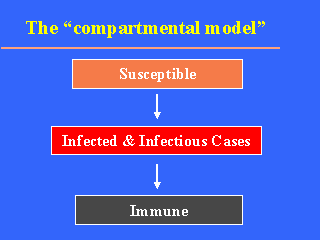
"compartmental model" (slide). According to this, all individuals of a
population belong to one of three categories or "compartments": a/ susceptible,
b/ infected and infectious, and c/ recovered and immune. As models depict the most essential elements of the spread of an infection, several
assumptions must be made. The most important ones usually are: a/ the latent period (from
the point of infection to the beginning of the infectious period) is negligible, b/ the
duration of infectivity is identical to that of clinical disease, c/ after recovery
everyone becomes immune and stays immune, d/ there is no degree of infectiousness (people
are either infectious or not), e/ the population is closed, i.e. no one enters (births,
immigration) or leaves (deaths, emigration), f/ everyone in the population has the same
chances to meet everyone else (homogeneous mixing). More elaborate models can, in some extent, account for factors such as latent period,
birth rate, period after birth with maternal antibodies, death rate, disease induced
mortality, loss of immunity, different mixing patterns among population groups, seasonal
variations in transmission rates etc.
|