This lab is concerned with several ways to compute eigenvalues and eigenvectors for a real matrix. All methods for computing eigenvalues and eigenvectors are iterative in nature, except for very small matrices. We begin with a short discussion of eigenvalues and eigenvectors, and then go on to the power method and inverse power methods. These are methods for computing a single eigenpair, but they can be modified to find several. We then look at shifting, which is an approach for computing one eigenpair whose eigenvalue is close to a specified value. We then look at the QR method, the most efficient method for computing all the eigenvalues at once. In the extra credit exercise, we see that the roots of a polynomial are easily computed by constructing the companion matrix and computing its eigenvalues.
This lab will take three sessions.
For any square ![]() matrix
matrix ![]() ,
consider the equation
,
consider the equation
![]() . This is a polynomial
equation of degree
. This is a polynomial
equation of degree ![]() in the variable
in the variable ![]() so there
are exactly
so there
are exactly ![]() complex roots (counting multiplicities) that satisfy
the equation. If
the matrix
complex roots (counting multiplicities) that satisfy
the equation. If
the matrix ![]() is real, then the complex roots occur in conjugate
pairs. The roots are known as ``eigenvalues'' of
is real, then the complex roots occur in conjugate
pairs. The roots are known as ``eigenvalues'' of ![]() .
Interesting questions include:
.
Interesting questions include:
If ![]() is an eigenvalue of
is an eigenvalue of ![]() , then
, then
![]() is a singular matrix, and therefore there is at least one nonzero
vector
is a singular matrix, and therefore there is at least one nonzero
vector ![]() with the property that
with the property that
![]() .
This equation is usually written
.
This equation is usually written
Interesting questions about eigenvectors include:
Some useful facts about the eigenvalues ![]() of a
matrix
of a
matrix ![]() :
:
If a vector ![]() is an exact eigenvector of a matrix
is an exact eigenvector of a matrix ![]() , then it
is easy to determine the value of the associated eigenvalue: simply
take the ratio of a component of
, then it
is easy to determine the value of the associated eigenvalue: simply
take the ratio of a component of
![]() and
and ![]() , for
any index
, for
any index ![]() that you like. But suppose
that you like. But suppose ![]() is only an
approximate eigenvector, or worse yet, just a wild guess. We could
still compute the ratio of corresponding components for some index,
but the value we get will vary from component to component. We might
even try computing all the ratios, and averaging them, or taking the
ratios of the norms. However, the preferred method for estimating the
value of an eigenvalue uses the so-called ``Rayleigh quotient.''
is only an
approximate eigenvector, or worse yet, just a wild guess. We could
still compute the ratio of corresponding components for some index,
but the value we get will vary from component to component. We might
even try computing all the ratios, and averaging them, or taking the
ratios of the norms. However, the preferred method for estimating the
value of an eigenvalue uses the so-called ``Rayleigh quotient.''
The Rayleigh quotient of a matrix ![]() and vector
and vector ![]() is
is
 |
|||
 |
If ![]() happens to be an eigenvector of the matrix
happens to be an eigenvector of the matrix ![]() , the the
Rayleigh quotient must equal its eigenvalue. (Plug
, the the
Rayleigh quotient must equal its eigenvalue. (Plug ![]() into the
formula and you will see why.) When the real vector
into the
formula and you will see why.) When the real vector ![]() is an
approximate eigenvector of
is an
approximate eigenvector of ![]() , the Rayleigh quotient is a very
accurate estimate of the corresponding eigenvalue. Complex
eigenvalues and eigenvectors require a little care because the dot
product involves multiplication by the conjugate transpose. The
Rayleigh quotient remains a valuable tool in the complex case, and
most of the facts remain true.
, the Rayleigh quotient is a very
accurate estimate of the corresponding eigenvalue. Complex
eigenvalues and eigenvectors require a little care because the dot
product involves multiplication by the conjugate transpose. The
Rayleigh quotient remains a valuable tool in the complex case, and
most of the facts remain true.
If the matrix ![]() is symmetric, then all eigenvalues
are real, and the Rayleigh quotient satisfies the following inequality.
is symmetric, then all eigenvalues
are real, and the Rayleigh quotient satisfies the following inequality.
function r = rayleigh ( A, x )
% r = rayleigh ( A, x )
% comments

% your name and the date
Be sure to include comments describing the input and output parameters and the purpose of the function.
       x          R(A,x)
  [ 3; 2; 1]       4.5
  [ 1; 0; 1]     __________    (is an eigenvector)
  [ 0; 1; 1]     __________    (is an eigenvector)
  [ 1;-2; 0]     __________    (is an eigenvector)
  [ 1; 1; 1]     __________
  [ 0; 0; 1]     __________
Note: The superscript ![]() in the above expressions
does not refer to a power of
in the above expressions
does not refer to a power of ![]() , or to a component. The use of
superscript distinguishes it from the
, or to a component. The use of
superscript distinguishes it from the
![]() component,
component, ![]() , and the parentheses distinguish it from an exponent. It is
simply the
, and the parentheses distinguish it from an exponent. It is
simply the
![]() vector in a sequence.
vector in a sequence.
The Rayleigh quotient
![]() provides a way to approximate
eigenvalues from an approximate eigenvector. Now we have to figure out
a way to come up with an approximate eigenvector.
provides a way to approximate
eigenvalues from an approximate eigenvector. Now we have to figure out
a way to come up with an approximate eigenvector.
In many physical and engineering applications, the largest or the
smallest eigenvalue associated with a system represents the dominant
and most interesting mode of behavior. For a bridge or support
column, the smallest eigenvalue might reveal the maximum load, and the
eigenvector represents the shape of the object at the instant of failure under this
load. For a concert hall, the smallest eigenvalue of the acoustic
equation reveals the lowest resonating frequency. For nuclear
reactors, the largest eigenvalue determines whether the reactor is
subcritical (![]() and reaction dies out), critical (
and reaction dies out), critical (![]() and
reaction is sustained), or supercritical (
and
reaction is sustained), or supercritical (![]() and reaction grows).
Hence, a simple means of approximating just one
extreme eigenvalue might be enough for some cases.
and reaction grows).
Hence, a simple means of approximating just one
extreme eigenvalue might be enough for some cases.
The ``power method'' tries to determine the largest magnitude eigenvalue, and the corresponding eigenvector, of a matrix, by computing (scaled) vectors in the sequence:
Note: As above, the superscript ![]() refers
to the
refers
to the
![]() vector in a sequence. When you write
Matlab code, you will typically denote both
vector in a sequence. When you write
Matlab code, you will typically denote both
![]() and
and
![]() with the same Matlab name x, and overwrite it each
iteration. In the signature lines specified below, xold is used
to denote
with the same Matlab name x, and overwrite it each
iteration. In the signature lines specified below, xold is used
to denote
![]() and x is used to denote
and x is used to denote
![]() and all subsequent iterates.
and all subsequent iterates.
If we include the scaling, and an estimate of the eigenvalue, the power method can be described in the following way.
function  [r, x, rHistory, xHistory] = power_method ( A, x ,maxNumSteps )
% [r, x, rHistory, xHistory] = power_method ( A, x ,maxNumSteps )
% comments

% your name and the date
   .
   .
   .
for k=1:maxNumSteps
   .
   .
   .
   r= ???  %Rayleigh quotient

   rHistory(k)=r;    % save Rayleigh quotient on each step
   xHistory(:,k)=x;  % save one eigenvector on each step
end
On exit, the xHistory variable will be a matrix whose columns are a (hopefully convergent) sequence of approximate dominant eigenvectors. The history variables rHistory and xHistory will be used to illustrate the progress that the power method is making and have no mathematical importance.
Note: It is usually the case that when writing code such as this that requires the Rayleigh quotient, I would ask that you use rayleigh.m, but in this case the Rayleigh quotient is so simple that it is probably better to just copy the code for it into power_method.m.
Using your power method code, try to determine the largest eigenvalue of the matrix eigen_test(1), starting from the vector [0;0;1]. (I have included the result for the first few steps to help you check your code out.)
  Step     Rayleigh q.    x(1)
  0          -4           0.0
  1         0.20455     0.12309
  2         2.19403     _____________________________
  3         __________  _____________________________
  4         __________  _____________________________
 10         __________  _____________________________
 15         __________  _____________________________
 20         __________  _____________________________
 25         __________  _____________________________
In addition, plot the progress of the method with the following commands
plot(rHistory);      title 'Rayleigh quotient vs. k'
plot(xHistory(1,:)); title 'Eigenvector first component vs. k'
Please send me these two plots with your summary.
function  [r, x, rHistory, xHistory] = power_method1 ( A, x , tol )
% [r, x, rHistory, xHistory] = power_method1 ( A, x , tol )
% comments

% your name and the date

maxNumSteps=10000;  % maximum allowable number of steps
You should have an if test with the Matlab return statement in it before the end of the loop. To determine when to stop iterating, add code to effect all three of the following criteria:
rold=r;  % save for convergence tests
xold=x;  % save for convergence tests
to save values for
disp('power_method1: Failed');
after the loop. Note: normally you would use an error
function call here, rather than disp, but for this lab you
will need to see the intermediate values in rHistory and
xHistory even when the method does not converge at all.
Matrix  Rayleigh q.    x(1)         no. iterations
  1      __________  __________      ____________
  2      __________  __________      ____________
  3      __________  __________      ____________
  4      __________  __________      ____________
  5      __________  __________      ____________
  6      __________  __________      ____________
  7      __________  __________      ____________
These matrices were chosen to illustrate different iterative behavior. Some converge quickly and some slowly, some oscillate and some don't. One does not converge. Generally speaking, the eigenvalue converges more rapidly than the eigenvector. You can check the eigenvalues of these matrices using the eig function. Plot the histories of Rayleigh quotient and first eigenvector component for all the cases. Send me the plots for cases 3, 5, and 7.
Matlab hint: The eig command will show you the eigenvectors as well as the eigenvalues of a matrix A, if you use the command in the form:
[ V, D ] = eig ( A )The quantities V and D are matrices, storing the n eigenvectors as columns in V and the eigenvalues along the diagonal of D.
The inverse power method reverses the iteration step of the power method. We write:
or, equivalently,
In other words, this looks like we are just doing a power method iteration, but now for the matrix
This means that we can freely choose to study the eigenvalue problem of
either ![]() or
or ![]() , and easily convert information
from one problem to the other. The difference is that
the inverse power iteration will find us the largest-in-magnitude eigenvalue
of
, and easily convert information
from one problem to the other. The difference is that
the inverse power iteration will find us the largest-in-magnitude eigenvalue
of ![]() , and that's the eigenvalue of
, and that's the eigenvalue of ![]() that's smallest in magnitude, while the plain power method
finds the eigenvalue of
that's smallest in magnitude, while the plain power method
finds the eigenvalue of ![]() that is largest in magnitude.
that is largest in magnitude.
The inverse power method iteration is given in the following algorithm.
Your file should have the signature:
function  [r, x, rHistory, xHistory] = inverse_power ( A, x, tol)
% [r, x, rHistory, xHistory] = inverse_power ( A, x, tol)
% comments

% your name and the date
Be sure to include a check on the maximum number of iterations (10000 is a good choice) so that a non-convergent problem will not go on forever.
[r x rHistory xHistory]=inverse_power(A,[0;0;1],1.e-8);Please include r and x in your summary. How many steps did it take?
[rp xp rHp xHp]=power_method1(inv(A),[0;0;1],1.e-8);You should find that r is close to 1/rp, that x and xp are close, and that xHistory and xHp are close. (You should not expect rHistory and 1./rHp to agree in the early iterations.) If these relations are not true, you have an error somewhere. Fix it before continuing. Warning: the two methods may take slightly different numbers of iterations. Compare xHistory and xHp only for the common iterations.
% choose the sign of x so that the dot product xold'*x >0
factor=sign(xold'*x);
if factor==0
  factor=1;
end
x=factor*x;
Matrix  Rayleigh q.    x(1)         no. iterations
  1     __________  __________      ____________
  2     __________  __________      ____________
  3     __________  __________      ____________
  4     __________  __________      ____________
  5     __________  __________      ____________
  6     __________  __________      ____________
  7     __________  __________      ____________
Be careful! One of these still does not converge. We could use a procedure similar to this exercise to discover and fix that one, but it is more complicated and conceptually similar, so we will not investigate it.
It is common to need more than one eigenpair, but not all eigenpairs. For example, finite element models of structures often have upwards of a million degrees of freedom (unknowns) and just as many eigenvalues. Only the lowest few are of practical interest. Fortunately, matrices arising from finite element structural models are typically symmetric and negative definite, so the eigenvalues are real and negative and the eigenvectors are orthogonal to one another.
For the remainder of this section, and this section only, we will be assuming that the matrix whose eigenpairs are being sought is symmetric so that the eigenvectors are orthogonal.
If you try to find two eigenvectors by using the power method (or the inverse power method) twice, on two different vectors, you will discover that you get two copies of the same dominant eigenvector. (The eigenvector with eigenvalue of largest magnitude is called ``dominant.'') Working smarter helps, though. Because the matrix is assumed symmetric, you know that the dominant eigenvector is orthogonal to the others, so you could use the power method (or the inverse power method) twice, forcing the two vectors to be orthogonal at each step of the way. This will guarantee they do not converge to the same vector. If this approach converges to anything, it probably converges to the dominant and ``next-dominant'' eigenvectors and their associated eigenvalues.
We considered orthogonalization in Lab 7 and we wrote a function called modified_gs.m. You can use your copy or mine for this lab. You will recall that this function regards the vectors as columns of a matrix: the first vector is the first column of a matrix X, the second is the second column, etc. Be warned that this function will sometimes return a matrix with fewer columns than the one it is given. This is because the original columns were not a linearly independent set. Code for real problems would need to recognize and repair this case, but it is not necessary for this lab.
The power method applied to several vectors can be described in the following algorithm:
Note: There is no guarantee that the eigenvectors that you find are the ones with largest magnitude eigenvalues! It is possible that your starting vectors were themselves orthogonal to one or more eigenvectors, and you will never recover eigenvectors that are not spanned by the initial ones. In applications, estimates of the inertia of the matrix can be used to mitigate this problem. See, for example, https://en.wikipedia.org/wiki/Sylvester%27s_law_of_inertia for a discussion of inertia of a matrix and how it can be used.
In the following exercise, you will write a Matlab function to carry out this procedure to find several eigenpairs for a symmetric matrix. The initial set of eigenvectors will be represented as columns of a Matlab matrix V.
function  [R, V, numSteps] = power_several ( A, V , tol )
% [R, V, numSteps] = power_several ( A, V , tol )
% comments

% your name and the date
to implement the algorithm described above.
d=sign(diag(Vold'*V));       % find signs of dot product of columns
D=diag(d);                   % diagonal matrix with +-1
V=V*D;                       % Transform V
  V = [ 0  0
        0  0
        0  0
        0  0
        0  1
        1  0];
What are the eigenvalues and eigenvectors? How many iterations are needed?
V=[0  0  0  0  0  1
   0  0  0  0  1  0
   0  0  0  1  0  0
   0  0  1  0  0  0
   0  1  0  0  0  0
   1  0  0  0  0  0 ];
What are the six eigenvalues? How many iterations were needed?
A major limitation of the power method is that it can only find the
eigenvalue of largest magnitude. Similarly, the inverse power iteration
seems only able to find the eigenvalue of smallest magnitude. Suppose,
however, that you want one (or a few) eigenpairs with eigenvalues that
are away from the extremes? Instead of working with
the matrix ![]() , let's work with the matrix
, let's work with the matrix
![]() , where
we have shifted the matrix by adding
, where
we have shifted the matrix by adding ![]() to every diagonal entry.
This shift makes a world of difference.
to every diagonal entry.
This shift makes a world of difference.
We already said the inverse power method finds the eigenvalue of smallest
magnitude. Denote the smallest eigenvalue of
![]() by
by
![]() . If
. If ![]() is an eigenvalue of
is an eigenvalue of
![]() then
then
![]() is singular. In other words,
is singular. In other words,
![]() is an eigenvalue
of
is an eigenvalue
of ![]() , and is the eigenvalue of
, and is the eigenvalue of ![]() that is closest to
that is closest to ![]() .
.
In general, the idea of shifting allows us to focus the attention of the inverse power method on seeking the eigenvalue closest to any particular value we care to name. This also means that if we have an estimated eigenvalue, we can speed up convergence by using this estimate in the shift. Although various strategies for adjusting the shift during the iteration are known, and can result in very rapid convergence, we will be using a constant shift.
We are not going to worry here about the details or the expense of shifting and refactoring the matrix. (A real algorithm for a large problem would be very concerned about this!) Our simple-minded method algorithm for the shifted inverse power method looks like this:
function  [r, x, numSteps] = shifted_inverse ( A, x, shift, tol)
% [r, x, numSteps] = shifted_inverse ( A, x, shift, tol)
% comments

% your name and the date
In the previous exercise, we used the backslash division operator. This is another example where the matrix could be factored first and then solved many times, with a possible time savings.
The value of the shift is at the user's disposal, and there is no
good reason to stick with the initial (guessed) shift. If it
is not too expensive to re-factor the matrix
![]() , then
the shift can be reset after each iteration of after a set of
n iterations, for n fixed.
, then
the shift can be reset after each iteration of after a set of
n iterations, for n fixed.
One possible choice for ![]() would be to set it equal to the
current eigenvalue estimate on each iteration. The result of this
choice is an algorithm that converges at an extremely fast rate, and
is the predominant method in practice.
would be to set it equal to the
current eigenvalue estimate on each iteration. The result of this
choice is an algorithm that converges at an extremely fast rate, and
is the predominant method in practice.
So far, the methods we have discussed seem suitable for finding one or a few eigenvalues and eigenvectors at a time. In order to find more eigenvalues, we'd have to do a great deal of special programming. Moreover, these methods are surely going to have trouble if the matrix has repeated eigenvalues, distinct eigenvalues of the same magnitude, or complex eigenvalues. The ``QR method'' is a method that handles these sorts of problems in a uniform way, and computes all the eigenvalues, but not the eigenvectors, at one time.
It turns out that the QR method is equivalent to the power method starting with a basis of vectors and with Gram-Schmidt orthogonalization applied at each step, as you did in Exercise 6. A nice explanation can be found in Prof. Greg Fasshauer's class notes. http://www.math.iit.edu/~fass/477577_Chapter_11.pdf
The QR method can be described in the following way.
The sequence of matrices ![]() is orthogonally similar
to the original matrix
is orthogonally similar
to the original matrix ![]() , and hence has the same eigenvalues.
This is because
, and hence has the same eigenvalues.
This is because
![]() , and
, and
![]() .
.
In Lab 7, you wrote the function gs_factor.m, that uses the modified Gram-Schmidt method to into the product of an orthogonal matrix, Q, and an upper-triangular matrix, R. You will be using this function in this lab. Everything in this lab could be done using the Matlab qr function or your h_factor.m function from Lab 7, but you should use gs_factor for this lab.
function  [e,numSteps] = qr_method ( A, tol)
% [e,numSteps] = qr_method ( A, tol)
% comments

% your name and the date
e is a vector of eigenvalues of A. Since the lower triangle of the matrix
where
  Matrix   largest & smallest Eigenvalues   Number of steps
  1           _________ _________           _________
  2           _________ _________           _________
  3           _________ _________           _________
  4           _________ _________           _________
  skip no. 5
  6           _________ _________           _________
  7           _________ _________           _________
Serious implementations of the QR method do not work the way our version works. The code resembles the code for the singular value decomposition you will see in the next lab and the matrices Q and R are never explicitly constructed. The algorithm also uses shifts to try to speed convergence and ceases iteration for already-converged eigenvalues.
In the following section we consider the question of convergence of the basic QR algorithm.
Throughout this lab we have used a very simple convergence criterion,
and you saw in the previous exercise that this convergence criterion
can result in errors that are too large.
In general, convergence is a difficult subject and fraught
with special cases and exceptions to rules. To give you a flavor of
how convergence might be reliably addressed, we consider the case of
the QR algorithm applied to a real, symmetric matrix, ![]() , with distinct
eigenvalues, no two of which are the same in magnitude. For such
matrices, the following theorem can be shown.
, with distinct
eigenvalues, no two of which are the same in magnitude. For such
matrices, the following theorem can be shown.
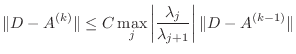
Theorem Let ![]() be a real symmetric matrix of order n and
let its eigenvalues satisfy
be a real symmetric matrix of order n and
let its eigenvalues satisfy
Then the iterates
The theorem points out a method for detecting convergence. Supposing you
start out with a matrix ![]() satisfying the above conditions, and you
call the matrix at the
satisfying the above conditions, and you
call the matrix at the
![]() iteration
iteration ![]() . If
. If ![]() denotes the matrix consisting only of the diagonal entries of
denotes the matrix consisting only of the diagonal entries of ![]() ,
then the Frobenius norm of
,
then the Frobenius norm of
![]() must go to zero as a power
of
must go to zero as a power
of
![]() , and if
, and if ![]() is the diagonal
matrix with the true eigenvalues on its diagonal, then
is the diagonal
matrix with the true eigenvalues on its diagonal, then ![]() must
converge to
must
converge to ![]() as a geometric series with ratio
as a geometric series with ratio ![]() .
In the following algorithm, the
diagonal entries of
.
In the following algorithm, the
diagonal entries of ![]() (these converge to the eigenvalues) will be the
only entries considered. The off-diagonal entries converge to zero, but
there is no need to make them small so long as the eigenvalues
are converged.
(these converge to the eigenvalues) will be the
only entries considered. The off-diagonal entries converge to zero, but
there is no need to make them small so long as the eigenvalues
are converged.
The following algorithm includes a convergence estimate as part of the QR algorithm.
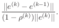
Return to step 2 if it exceeds the required tolerance.
The reason is that if
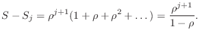
You may wonder where the denominator ![]() came from. Consider
the geometric series
came from. Consider
the geometric series
Truncating this series at the
But,
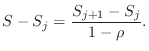
Thus, the error made in truncating a geometric series is the difference of two partial sums divided by
function [e, numSteps]=qr_convergence(A,tol)
% [e, numSteps]=qr_convergence(A,tol)
% comments

% your name and the date
Modify the code to implement the above algorithm.
norm(sort(e)-sort(eMatlab))/norm(e)where e is the vector of eigenvalues from qr_convergence?
A = [ .01  1
      -1  .01];
It should fail. Explain how you know it failed and what went wrong.
Have you ever wondered how all the roots of a polynomial can be
found? It is fairly easy to find the largest and smallest real roots
using, for example, Newton's method, but then what? If you know
a root ![]() exactly, of course, you can eliminate it by dividing by
exactly, of course, you can eliminate it by dividing by
![]() (called ``deflation''), but in the numerical world you never
know the root exactly, and deflation with an inexact root can introduce
large errors. Eigenvalues come to the rescue.
(called ``deflation''), but in the numerical world you never
know the root exactly, and deflation with an inexact root can introduce
large errors. Eigenvalues come to the rescue.
Suppose you are given a monic (![]() ) polynomial of degree
) polynomial of degree ![]()
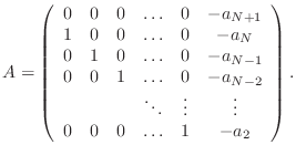
It is easy to see that
function r=myroots(a)
% r=myroots(a)
% comments

% your name and the date
that will take a vector of coefficients and find all the roots of the polynomial