We have seen that the PLU factorization can be used to solve a linear system provided that the system is square, and that it is nonsingular, and that it is not too badly conditioned. However, if we want to handle problems with a bad condition number, or that are singular, or even rectangular, we are going to need to come up with a different approach. In this lab, we will look at two versions of the QR factorization:
where
The QR factorization will form the basis of a method for finding eigenvalues of matrices in a later lab. It can also be used to solve linear systems, especially poorly-conditioned ones that the PLU factorization can have trouble with. In addition, topics such as the Gram Schmidt method and Householder matrices have application in many other contexts.
This lab will take two sessions.
Definition: An ``orthogonal matrix'' is a real matrix whose inverse is equal to its transpose.
By convention, an orthogonal matrix is usually denoted by the
symbol ![]() . The definition of an orthogonal matrix immediately
implies that
. The definition of an orthogonal matrix immediately
implies that
One way to interpret this equation is that the columns of the matrix
and the fact that
you should be able to deduce that, for orthogonal matrices,
If I multiply a two-dimensional vector ![]() by
by ![]() then
its
then
its ![]() norm doesn't change,
and so
norm doesn't change,
and so ![]() must lie on the circle whose radius is
must lie on the circle whose radius is
![]() . In
other words,
. In
other words, ![]() is
is
![]() rotated around the origin by some angle, or reflected through
the origin or about a diameter. That means that a two-dimensional orthogonal
matrix represents a rotation or reflection. Even in
N dimensions, orthogonal matrices are often called rotations.
rotated around the origin by some angle, or reflected through
the origin or about a diameter. That means that a two-dimensional orthogonal
matrix represents a rotation or reflection. Even in
N dimensions, orthogonal matrices are often called rotations.
When matrices are complex, the term ``unitary'' is an analog to
``orthogonal.'' A matrix is unitary if
![]() , where the
, where the ![]() superscript refers to the ``Hermitian'' or ``conjugate-transpose''
of the matrix. In Matlab, the prime operator implements the
Hermitian and the dot-prime operator implements the transpose.
A real matrix that is unitary is orthogonal.
superscript refers to the ``Hermitian'' or ``conjugate-transpose''
of the matrix. In Matlab, the prime operator implements the
Hermitian and the dot-prime operator implements the transpose.
A real matrix that is unitary is orthogonal.
The ``Gram Schmidt method'' can be thought of as a process that
analyzes a set of vectors ![]() , producing a
(possibly smaller) set of vectors
, producing a
(possibly smaller) set of vectors ![]() that: (a) span the
same space; (b) have unit
that: (a) span the
same space; (b) have unit ![]() norm; and, (c) are pairwise orthogonal.
Note that if we can produce such a set of vectors, then we can
easily answer several important questions.
For example, the size of the set
norm; and, (c) are pairwise orthogonal.
Note that if we can produce such a set of vectors, then we can
easily answer several important questions.
For example, the size of the set ![]() tells us whether the set
tells us whether the set
![]() was linearly independent, and the dimension of the space
spanned and the rank of a matrix constructed from the vectors.
And of course, the vectors in
was linearly independent, and the dimension of the space
spanned and the rank of a matrix constructed from the vectors.
And of course, the vectors in ![]() are the orthonormal basis
we were seeking. So you should believe that being able to compute
the vectors
are the orthonormal basis
we were seeking. So you should believe that being able to compute
the vectors ![]() is a valuable ability.
is a valuable ability.
We will be using the Gram-Schmidt process to factor a matrix, but the process itself pops up repeatedly whenever sets of vectors must be made orthogonal. You may see it, for example, in Krylov space methods for iteratively solving systems of equations and for eigenvalue problems.
In words, the Gram-Schmidt process goes like this:
Classical Gram-Schmidt algorithm
|
|
|
for k = 1 to |
|
|
|
for |
|
|
|
|
| end |
|
|
|
if |
|
|
|
|
| end |
| end |
You should be able to match this algorithm to the previous verbal
description. Can you see how the ![]() norm of a vector is being computed?
Note that the auxilliary vector
norm of a vector is being computed?
Note that the auxilliary vector
![]() is needed here because without
it the vector
is needed here because without
it the vector
![]() would be changed during the loop on
would be changed during the loop on ![]() instead of only after the loop is complete.
instead of only after the loop is complete.
The Gram-Schmidt algorithm as described above can be subject to errors due to roundoff when implemented on a computer. Nonetheless, in the first exercise you will implement it and confirm that it works well in some cases. In the subsequent exercise, you will examine an alternative version that has been modifed to reduce its sensitivity to roundoff error.
function Q = unstable_gs ( X )
% Q = unstable_gs( X )
% more comments

% your name and the date
Assume the ![]() vectors are stored as columns of the
matrix X. Be sure you understand this data structure
because it is a potential source of confusion. In the
algorithm description above, the
vectors are stored as columns of the
matrix X. Be sure you understand this data structure
because it is a potential source of confusion. In the
algorithm description above, the ![]() vectors are
members of a set
vectors are
members of a set ![]() , but here these vectors are
stored as the columns of a matrix X. Similarly,
the vectors in the set
, but here these vectors are
stored as the columns of a matrix X. Similarly,
the vectors in the set ![]() are stored as the
columns of a matrix Q. The first
column of X corresponds to the vector
are stored as the
columns of a matrix Q. The first
column of X corresponds to the vector ![]() , so that
the Matlab expression X(k,1) refers to the
, so that
the Matlab expression X(k,1) refers to the
![]() component of the vector
component of the vector ![]() , and the Matlab expression
X(:,1) refers to the Matlab column vector corresponding
to
, and the Matlab expression
X(:,1) refers to the Matlab column vector corresponding
to ![]() . Similarly for the
other columns.
Include your code with your summary report.
. Similarly for the
other columns.
Include your code with your summary report.
  X = [ 1  1  1
        0  1  1
        0  0  1 ]
You should be able to see that the correct result is the identity matrix.
If you do not get the identity matrix, find your bug before continuing.
  X = [ 1  1  1
        1  1  0
        1  0  0 ]
The columns of Q should have
  X = [  2  -1   0
        -1   2  -1
         0  -1   2
         0   0  -1 ]
If your code is working correctly, you should compute approximately:
      [  0.8944   0.3586   0.1952
        -0.4472   0.7171   0.3904
         0.0000  -0.5976   0.5855
         0.0000   0.0000  -0.6831 ]
You should verify that the columns of Q have It would be foolish to use the unstable form of the Gram-Schmidt factorization when the modified Gram-Schmidt algorithm is only slightly more complicated. The modified Gram-Schmidt algorithm can be described in the following way.
Modified Gram-Schmidt algorithm
|
|
|
for k = 1 to |
|
|
|
for |
|
|
|
|
| end |
|
|
|
if |
|
|
|
|
| end |
| end |
The modification seems pretty minor. In exact arithmetic, it makes no
difference at all. Suppose, however, that because of roundoff errors a
``little bit'' of
![]() slips into
slips into
![]() . In the original
algorithm the ``little bit'' of
. In the original
algorithm the ``little bit'' of
![]() will cause
will cause
![]() to be slightly less accurate
than
to be slightly less accurate
than
![]() because there is a ``more of''
because there is a ``more of''
![]() inside
inside
![]() than
there is inside
than
there is inside
![]() . In the next exercise you will see that
the modified algorithm can be less affected by roundoff than the original
one.
. In the next exercise you will see that
the modified algorithm can be less affected by roundoff than the original
one.
function Q = modified_gs( X )
% Q = modified_gs( X )
% more comments

% your name and the date
Your code should be something like unstable_gs.m.
We need to take a closer look at the Gram-Schmidt process. Recall how
the process of Gauss elimination could actually be regarded as a process
of factorization. This insight enabled us to solve many other problems.
In the same way, the Gram-Schmidt process is actually carrying out
a different factorization that will give us the key to other problems.
Just to keep our heads on straight, let me point out that we're
about to stop thinking of ![]() as a bunch of vectors, and instead
regard it as a matrix. Since it is traditional for matrices
to be called
as a bunch of vectors, and instead
regard it as a matrix. Since it is traditional for matrices
to be called ![]() that's what we'll call our set of vectors from
now on.
that's what we'll call our set of vectors from
now on.
Now, in the Gram-Schmidt algorithm, the numbers that we called
![]() and
and ![]() , that we computed,
used, and discarded, actually record important information. They can
be regarded as the nonzero elements of an upper triangular matrix
, that we computed,
used, and discarded, actually record important information. They can
be regarded as the nonzero elements of an upper triangular matrix
![]() . The Gram-Schmidt process actually produces a
factorization of the matrix
. The Gram-Schmidt process actually produces a
factorization of the matrix ![]() of the form:
of the form:
Here, the matrix
function [ Q, R ] = gs_factor ( A )
% [ Q, R ] = gs_factor ( A )
% more comments

% your name and the date
Include a copy of your code with your summary.
Recall: [Q,R]=gs_factor is the syntax that Matlab uses to return two matrices from the function. When calling the function, you use the same syntax:
[Q,R]=gs_factor(...When you use this syntax, it is OK (but not a great idea) to leave out the comma between the Q and the R but leaving out that comma is a syntax error in the signature line of a function m-file. I recommend you use the comma all the time.
  A = [ 1  1  1
        1  1  0
        1  0  0 ]
Compare the matrix Q computed using gs_factor with
the matrix computed using modified_gs. They should be the same.
Check that
  A = [ 0   0   1
        1   2   3
        5   8  13
       21  34  55 ]
It turns out that it is possible to take a given vector
![]() and a given integer
and a given integer ![]() and find a matrix
and find a matrix ![]() so that the product
so that the product
![]() is proportional to the vector
is proportional to the vector
 .
That is, it is possible to
find a matrix
.
That is, it is possible to
find a matrix ![]() that ``zeros out'' all but the
that ``zeros out'' all but the
![]() th
entry of
th
entry of
![]() . (In this section, we will be concerned
primarily with the case
. (In this section, we will be concerned
primarily with the case ![]() .) The matrix is given by
.) The matrix is given by
 |
|||
 |
|||
There is a way to use this idea to
take any column of a matrix and make those entries below
the diagonal entry be zero, as is done in the
![]() th
step
of Gaußian factorization. This will lead to another
matrix factorization.
th
step
of Gaußian factorization. This will lead to another
matrix factorization.
Consider a column vector of length ![]() split into two
split into two
![$\displaystyle \mathbf{b}=
\left[\begin{array}{c}b_1 b_2 \vdots b_{k-1}\\
\overline{\hspace*{3em}}\\
b_k b_{k+1} \vdots b_n\end{array}\right],
$](img80.png)
and denote part of
![$\displaystyle \mathbf{d}=
\left[\begin{array}{c}
d_1 d_{2} \vdots d_{n-k+...
...right]
=\left[\begin{array}{c}
b_k b_{k+1} \vdots b_n\end{array}\right].
$](img83.png)
Construct an
![$\displaystyle {\huge\left[\begin{array}{c\vert c} I & 0 [-10pt] \rule{20pt}{...
...rline{\hspace*{3em}} \Vert\mathbf{d}\Vert 0 \vdots 0\end{array}\right].$](img86.png) |
![$\displaystyle H=\left[\begin{array}{cc} I & 0 0 & H_d\end{array}\right]$](img87.png) |
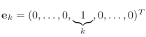
The algorithm for computing ![]() involves constructing a
involves constructing a
![]() -vector
-vector
![]() , the same size as
, the same size as
![]() .
Once
.
Once
![]() has been constructed, it will be expanded
to a
has been constructed, it will be expanded
to a ![]() -vector
-vector
![]() by adding
by adding ![]() leading zeros.
leading zeros.
![$\displaystyle \mathbf{w}=\left[\begin{array}{c} 0 \vdots 0 v_1 v_2 \vdots v_{n-k+1} \end{array}\right]$](img93.png) |
![$\displaystyle H=\left[\begin{array}{cc} I & 0 0 & H_d\end{array}\right].$](img95.png) |
The following algorithm for constructing
![]() and
and
![]() includes a choice of sign that minimizes roundoff errors. This
choice results in the sign of
includes a choice of sign that minimizes roundoff errors. This
choice results in the sign of
![]() in
(2) being either positive or negative.
in
(2) being either positive or negative.
Constructing a Householder matrix
![$ \mathbf{w}=
\left[\begin{array}{c}0\\
\vdots\\
0\\
\mathbf{v}\end{array}\right].$](img106.png)
The vector
![]() is specified above in (1)
and clearly is a unit vector. It is hard to see that the vector
is specified above in (1)
and clearly is a unit vector. It is hard to see that the vector
![]() as defined in the algorithm above is a unit vector satisfying
(1). The calculation confirming that
as defined in the algorithm above is a unit vector satisfying
(1). The calculation confirming that
![]() is a
unit vector is presented here. You should look carefully at the
algorithm to convince yourself that
is a
unit vector is presented here. You should look carefully at the
algorithm to convince yourself that
![]() also satsifies (1).
also satsifies (1).
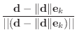
Suppose you are given a vector
![]() . Define
. Define
 |
||
 |
||
 |
||
 |
||
 |
In the following exercise you will write a Matlab function to implement this algorithm.
function H = householder(b, k)
% H = householder(b, k)
% more comments

% your name and the date

n = size(b,1);
if size(b,2) ~= 1
  error('householder: b must be a column vector');
end

d(:,1) = b(k:n);
if d(1)>=0
  alpha = -norm(d);
else
  alpha =  norm(d);
end
H = eye(n);otherwise, complete the above algorithm.
This householder function can be used for
the QR factorization of a matrix by proceeding
through a series of partial factorizations
![]() , where
, where ![]() is
the identity matrix, and
is
the identity matrix, and ![]() is the matrix
is the matrix ![]() .
When we begin the
.
When we begin the
![]() step of factorization, our factor
step of factorization, our factor
![]() is only upper triangular in columns 1 to
is only upper triangular in columns 1 to ![]() .
Our goal on the
.
Our goal on the ![]() -th step is to find a better factor
-th step is to find a better factor
![]() that is upper triangular through column
that is upper triangular through column ![]() .
If we can do this process
.
If we can do this process ![]() times, we're done.
Suppose, then, that we've partially factored the matrix
times, we're done.
Suppose, then, that we've partially factored the matrix ![]() , up
to column
, up
to column ![]() . In other words, we have a factorization
. In other words, we have a factorization
for which the matrix
and we're guaranteed that
For a rectangular ![]() by
by ![]() matrix
matrix ![]() , the
Householder QR factorization has the form
, the
Householder QR factorization has the form
where the matrix
If the matrix ![]() is not square, then this definition is
different from the Gram-Schmidt factorization we discussed before.
The obvious difference is the shape of the factors.
Here, it's the
is not square, then this definition is
different from the Gram-Schmidt factorization we discussed before.
The obvious difference is the shape of the factors.
Here, it's the ![]() matrix that is square. The other difference,
which you'll have to take on faith, is that the Householder
factorization is generally more accurate (smaller arithmetic
errors), and easier to define compactly.
matrix that is square. The other difference,
which you'll have to take on faith, is that the Householder
factorization is generally more accurate (smaller arithmetic
errors), and easier to define compactly.
Householder QR Factorization Algorithm:
| Q = I; |
| R = A; |
| for k = 1:min(m,n) |
| Construct the Householder matrix H for column k of the matrix R; |
| Q = Q * H'; |
| R = H * R; |
| end |
function [ Q, R ] = h_factor ( A )
% [ Q, R ] = h_factor ( A )
% more comments

% your name and the date
Use the routine householder.m in order to compute the H matrix that you need at each step.
A = [ 0 1 1
      1 1 1
      0 0 1 ]
You should see that simply interchanging the first and second
rows of A turns it into an upper triangular matrix.
The matrix Q that you get is equivalent to a permutation
matrix, execpt possibly with (-1) in some positions.
You can guess what
the solution is. Be sure that Q*R is A.
If we have computed the Householder QR factorization of a matrix
without encountering any singularities, then it is easy to solve linear
systems. We use the property of the ![]() factor that
factor that
![]() :
:
function x = h_solve ( Q, R, b )
% x = h_solve ( Q, R, b )
% more comments

% your name and the date
The matrix R is upper triangular, so you can use u_solve to solve (3) above. Assume that the QR factors come from the h_factor routine. Set up your code to compute
When you think your solver is working, test it out on a system as follows:
    n = 5;
    A = magic ( n );
    x = [ 1 : n ]';
    b = A * x;
    [ Q, R ] = h_factor ( A );
    x2 = h_solve ( Q, R, b );
    norm(x - x2)/norm(x) % should be close to zero.
Now you know another way to solve a square linear system. It turns out that you can also use the QR algorithm to solve non-square systems, but that task is better left to the singular value decomposition in a later lab.
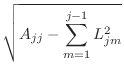
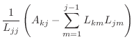
In the case that the matrix ![]() is symmetric positive definite, then
is symmetric positive definite, then
![]() can be factored uniquely as
can be factored uniquely as ![]() , where
, where ![]() is a lower-triangular
matrix with positive values on the diagonal.
This factorization is called the ``Cholesky factorization'' and is
both highly efficient (in terms of both storage and time) and also
not very sensitive to roundoff errors.
is a lower-triangular
matrix with positive values on the diagonal.
This factorization is called the ``Cholesky factorization'' and is
both highly efficient (in terms of both storage and time) and also
not very sensitive to roundoff errors.
You can find more information about Cholesky factorization in your text and also in a Wikipedia article http://en.wikipedia.org/wiki/Cholesky_decomposition.
 |
||
 for for |
function L=cholesky(A)
% L=cholesky(A)
% more comments

% your name and the date
N = 50;
A = rand(N,N);        % random numbers between 0 and 1
A = .5 * (A + A');    % force A to be symmetric
A = A + diag(sum(A)); % make A positive definite by Gershgorin
x = rand(N,1);        % solution
b = A*x;              % right side
![$\displaystyle H\mathbf{b}=H \left[\begin{array}{c}b_1 b_2 \vdots b_{k-1}\...
...rline{\hspace*{3em}} \Vert\mathbf{d}\Vert 0 \vdots 0\end{array}\right].$](img88.png)