The objects we work with in linear systems are vectors and matrices. In order to make statements about the size of these objects, and the errors we make in solutions, we want to be able to describe the ``sizes'' of vectors and matrices, which we do by using norms.
We then need to consider whether we can bound the size of the product of a matrix and vector, given that we know the ``size'' of the two factors. In order for this to happen, we will need to use matrix and vector norms that are compatible. These kinds of bounds will become very important in error analysis.
We will then consider the notions of forward error and backward error in a linear algebra computation.
We will then look at one useful matrix example: a tridiagonal matrix with well-known eigenvalues and eigenvectors.
This lab will take two sessions.
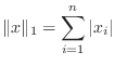
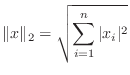
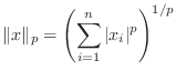
A vector norm assigns a size to a vector, in such a way that
scalar multiples do what we expect, and the triangle inequality is
satisfied. There are four common vector norms in ![]() dimensions:
dimensions:
To compute the norm of a vector ![]() in Matlab:
in Matlab:
   x1 = [ 4; 6; 7 ]
   x2 = [ 7; 5; 6 ]
   x3 = [ 1; 5; 4 ]
compute the vector norms, using the appropriate Matlab commands. Be sure your answers are reasonable.
        L1            L2            L Infinity

  x1    __________    __________    __________
  x2    __________    __________    __________
  x3    __________    __________    __________
A matrix norm assigns a size to a matrix, again, in such a way that scalar multiples do what we expect, and the triangle inequality is satisfied. However, what's more important is that we want to be able to mix matrix and vector norms in various computations. So we are going to be very interested in whether a matrix norm is compatible with a particular vector norm, that is, when it is safe to say:
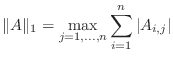
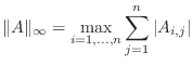
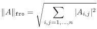
There are four common matrix norms and one ``almost'' norm:
Remark: This is not the same as the
where
where
Remark: This is not the same as the
Remark: This is the same as the
(only defined for a square matrix), where
To compute the norm of a matrix ![]() in Matlab:
in Matlab:
A matrix can be identified with a linear operator, and the norm of a linear operator is usually defined in the following way.
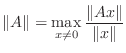
(It would be more precise to use
In order for a matrix norm to be consistent with the linear operator norm, you need to be able to say the following:
If a matrix norm is vector-bound to a particular vector norm, then the
two norms are guaranteed to be compatible. Thus, for any vector norm,
there is always at least one matrix norm that we can use. But that
vector-bound matrix norm is not always the only choice. In particular,
the ![]() matrix norm is difficult (time-consuming) to compute, but there
is a simple alternative.
matrix norm is difficult (time-consuming) to compute, but there
is a simple alternative.
Note that:
There is a theorem, though, that states that, for any matrix
   x1 = [ 4; 6; 7 ];
   x2 = [ 7; 5; 6 ];
   x3 = [ 1; 5; 4 ];
and each of the following matrices
A1 = [38   37   80
      53   49   49
      23   85   46];

A2 = [77   89   78
       6   34   10
      65   36   26];
Check that the compatibility condition (1) holds for
each case in the following table by computing the ratios
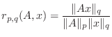
and filling in the following table. The third column should contain the letter ``S'' if the compatibility condition is satisfied and the letter ``U'' if it is unsatisfied.
Suggestion: I recommend you write a script m-file for this exercise. If you do, please include it with your summary.
Matrix  Vector
 norm    norm   S/U   r(A1,x1)   r(A1,x2)    r(A1,x3)    r(A2,x1)    r(A2,x2)    r(A2,x3)
  (p)     (q)

   1      1     ___   _________  __________  __________  __________  __________  __________
   1      2     ___   _________  __________  __________  __________  __________  __________
   1     inf    ___   _________  __________  __________  __________  __________  __________

   2      1     ___   _________  __________  __________  __________  __________  __________
   2      2     ___   _________  __________  __________  __________  __________  __________
   2     inf    ___   _________  __________  __________  __________  __________  __________

  inf     1     ___   _________  __________  __________  __________  __________  __________
  inf     2     ___   _________  __________  __________  __________  __________  __________
  inf    inf    ___   _________  __________  __________  __________  __________  __________

 'fro'    1     ___   _________  __________  __________  __________  __________  __________
 'fro'    2     ___   _________  __________  __________  __________  __________  __________
 'fro'   inf    ___   _________  __________  __________  __________  __________  __________
In the above text there is a statement that the spectral radius is not vector-bound with any norm, but that it ``almost'' is. In this section we will see by example what this means.
In the first place, let's try to see why it isn't vector-bound to
the ![]() norm. Consider the following false ``proof''.
Given a matrix
norm. Consider the following false ``proof''.
Given a matrix ![]() , for any vector
, for any vector ![]() , break it into a sum
of eigenvectors of
, break it into a sum
of eigenvectors of ![]() as
as
where
Why is this ``proof'' false? The error is in the
statement that all vectors can be expanded as sums of orthonormal eigenvectors.
If you knew, for example, that ![]() were positive definite and symmetric,
then, the eigenvectors of
were positive definite and symmetric,
then, the eigenvectors of ![]() would form an orthonormal basis and the
proof would
be correct. Hence the term ``almost.'' On the other hand, this
observation provides the counterexample.
would form an orthonormal basis and the
proof would
be correct. Hence the term ``almost.'' On the other hand, this
observation provides the counterexample.
A=[0.5  1   0   0   0   0   0
    0  0.5  1   0   0   0   0
    0   0  0.5  1   0   0   0
    0   0   0  0.5  1   0   0
    0   0   0   0  0.5  1   0
    0   0   0   0   0  0.5  1
    0   0   0   0   0   0  0.5]
You should recognize this as a Jordan block. Any matrix
can be decomposed into several such blocks by a change of basis.
It is a well-known fact that if the spectral radius of a matrix A is
smaller than 1.0 then
![]() .
.
The Euclidean norm (two norm) for matrices is a natural norm to use, but it has the disadvantage of requiring more computation time than the other norms. However, the two norm is compatible with the Frobenius norm, so when computation time is an issue, the Frobenius norm should be used instead of the two norm.
The two norm of a matrix is computed in Matlab as the largest singular value of the matrix. (See Quarteroni, Sacco, Saleri, p. 17-18, or a Wikipedia article http://en.wikipedia.org/wiki/Singular_value_decomposition for a discussion of singular values of a matrix.) We will visit singular values again in Lab 9 and you will see some methods for computing the singular values of a matrix. You will see in the following exercise that computing the singular value of a large matrix can take a considerable amount of time.
Matlab provides a ``stopwatch'' timer that measures elapsed time for a command. The command tic starts the stopwatch and the command toc prints (or returns) the time elapsed since the tic command. When using these commands, you must take care not to type them individually on different lines since then you would be measuring your own typing speed.
A=magic(1000); % DO NOT LEAVE THE SEMICOLON OUT!
tic;x=norm(A);tocto discover how long it takes to compute the two norm of A. (Be patient, this computation may take a while.) Please include both the value of x and the elapsed time in your summary. (You may be interested to note that x = sum(diag(A)) = trace(A) = norm(A,1) = norm(A,inf).)
A natural assumption to make is that the term ``error'' refers always
to the difference between the computed and exact ``answers.'' We are
going to have to discuss several kinds of error, so let's refer to
this first error as ``solution error'' or ``forward error.''
Suppose we want to solve a linear system of the form
![]() , (with
exact solution
, (with
exact solution ![]() ) and we computed
) and we computed
![]() . We
define the solution error as
. We
define the solution error as
![]() .
.
Usually the solution error cannot be computed, and we would
like a substitute whose behavior is acceptably close to that of
the solution error. One example would be during an iterative solution
process where we would like to monitor the progress of the iteration but
we do not yet have the solution and cannot compute the solution error.
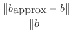
In this case, we are interested in the ``residual error'' or ``backward
error,'' which is defined by
![]() where, for convenience,
we have defined the variable
where, for convenience,
we have defined the variable
![]() to equal
to equal
![]() . Another way of looking at the residual error is
to see that it's telling us the difference between the right hand side
that would ``work'' for
. Another way of looking at the residual error is
to see that it's telling us the difference between the right hand side
that would ``work'' for
![]() versus the right
hand side we have.
versus the right
hand side we have.
If we think of the right hand side as being a target, and our solution procedure as determining how we should aim an arrow so that we hit this target, then
Case Residual large/small  xTrue   Error   large/small
 1   ________   _______   ______   _______   ________
 2   ________   _______   ______   _______   ________
 3   ________   _______   ______   _______   ________
 4   ________   _______   ______   _______   ________
The norms of the matrix and its inverse exert some limits on the relationship between the forward and backward errors. Assuming we have compatible norms:
and
Put another way,
It's often useful to consider the size of an error relative to the
true quantity. This quantity is sometimes multiplied by 100 and
expressed as a ``percentage.'' If the true solution is ![]() and we
computed
and we
computed
![]() , the relative solution error is defined as
, the relative solution error is defined as
 |
|||
 |
|||
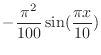
Actually, relative quantities are important beyond being ``easier
to understand.'' Consider the boundary value problem (BVP) for the ordinary
differential equation
[x,u]=bvp(10);
plot(x,u,x,sin(pi*x/10));
legend('computed solution','exact solution');
The two solutions curves should lie almost on top of one another.
You do not need to send me the plot.
sizes=[10 20 40 80 160 320 640];
for k=1:numel(sizes)
  [x,u]=bvp(sizes(k));
  error(k,1)=norm(u'-sin(pi*x/10));
  relative_error(k,1)=error(k,1)/norm(sin(pi*x/10));
end
disp([error(1:6)./error(2:7) ,  ...
      relative_error(1:6)./relative_error(2:7)])
                  Euclidean norm
          error ratio       relative error ratio
 10/ 20   ___________       ___________
 20/ 40   ___________       ___________
 40/ 80   ___________       ___________
 80/160   ___________       ___________
160/320   ___________       ___________
320/640   ___________       ___________
                  1 vector norm
          error ratio       relative error ratio
 10/ 20   ___________       ___________
 20/ 40   ___________       ___________
 40/ 80   ___________       ___________
 80/160   ___________       ___________
160/320   ___________       ___________
320/640   ___________       ___________
                  Infinity vector norm
          error ratio       relative error ratio
 10/ 20   ___________       ___________
 20/ 40   ___________       ___________
 40/ 80   ___________       ___________
 80/160   ___________       ___________
160/320   ___________       ___________
320/640   ___________       ___________
                Rate=h^2?

Euclidean     ____________
one           ____________
infinity      ____________
The reason that the ![]() and
and ![]() norms give different results is
that the dimension of the space,
norms give different results is
that the dimension of the space, ![]() creeps into the calculation. For
example, if a function is identically one,
creeps into the calculation. For
example, if a function is identically one, ![]() , then its
, then its ![]() norm,
norm,
![]() is one, but if a vector of dimension
is one, but if a vector of dimension ![]() has
all components equal to one, then its
has
all components equal to one, then its ![]() norm is
norm is ![]() . Taking
relative norms eliminates the dependence on
. Taking
relative norms eliminates the dependence on ![]() .
.
When you are doing your own research, you will have occasion to compare theoretical and computed convergence rates. When doing so, you may use tables such as those above. If you find that your computed convergence rates differ from the theoretical ones, before looking for some error in your theory, you should first check that you are using the correct norm!
It is a good idea to have several matrix examples at hand when you
are thinking about some method. One excellent example a class of
tridiagonal matrices that arise from second-order differential equations.
You saw matrices of this class in the previous lab in the section on
Discretizing a BVP.
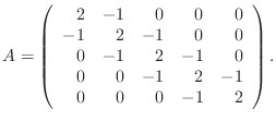
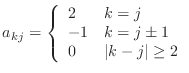
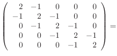
A ![]() matrix in this class is given as
matrix in this class is given as
function A=tridiagonal(N)
% A=tridiagonal(N) generates the tridiagonal matrix A

% your name and the date

A=zeros(N);
??? code corresponding to equation (4) ???
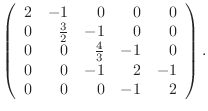
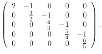
function A=rrs(A,j)
% A=rrs(A,j) performs one row reduction step for row j
% j must be between 2 and N

% your name and the date
N=size(A,1);
if (j<=1 | j>N)  % | means "or"
  j
  error('rrs: value of j must be between 2 and N');
end

factor=1/A(j-1,j-1);  % factor to multiply row (j-1) by

 ??? include code to multiply row (j-1) by factor and ???
 ??? add it to row (j).  Row (j-1) remains unchanged. ???
Check your work by comparing it with (6-8).
The
Laplace rule for computing the determinant of an ![]() matrix
matrix ![]() with entries
with entries ![]() is given by
is given by
 |
 |
Back to MATH2071 page.
 det
det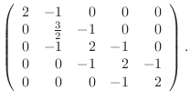
![$\displaystyle (A)=\left\{ \begin{array}{ll} a_{11} & N=1 [3pt] \sum_{j=1}^N a_{kj}\Delta_{kj} & N>1 \end{array}\right.$](img128.png)