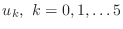
MATH2071: LAB 4: BVPs and PDEs
Introduction
The initial value problem for ordinary differential equations of the
previous labs is only one of the two major types of problem for
ordinary differential equations. The other type
is known as the ``boundary value problem'' (BVP).
A simple example of such a problem would describe the shape of a
rope hanging between two posts. We know the position of the
endpoints, and we have a second order differential equation
describing the shape. If the two conditions were both given at the
left endpoint, we'd know what to do right away. But how do we handle
this ``slight'' variation?
This lab is concerned with two of the most common approaches to solving
BVPs as well as a combined IVP-BVP for a partial differential equation.
The extra credit problem introduces a third approach to solving BVPs.
The discussion in this lab is limited to relatively simple approaches
in a single space dimension and is intended to give the flavor of these
approaches, each of which could easily be the subject of a full
semester's course. Except for the extra credit exercise, these methods
are easily extended to two and three space dimensions.
The approaches included in this lab are the following:
- The Finite Difference method (FDM),
- The Finite Element method (FEM),
- The Method of Lines, and,
- The Shooting method (extra credit).
Boundary Value Problems
A one-dimensional boundary value problem (BVP), is similar to an
initial value problem, except that the data we are given isn't
conveniently located at a starting point, but rather some is specified
at the left end point and some at the right. (We're also usually
thinking of the independent variable as representing space, rather
than time, in this setting).
We will be using the following problem as the illustrative example
for several of the following exercises.
The clothesline BVP: A rope is stretched between two
points. If the rope were weightless, or if it were rigid, it would lie along a
straight line; however, the rope has a weight and is elastic, so it
sags down slightly from its ideal linear shape. We wish to determine the curve
described by the rope. We will use the variable  to denote
horizontal distance and
to denote
horizontal distance and  to denote height of the rope
at the point
.
to denote height of the rope
at the point
.
Forces on a clothesline
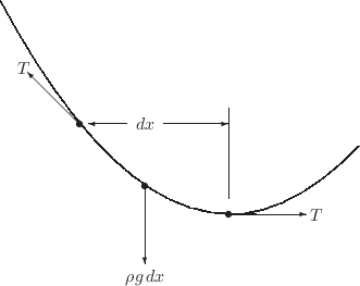
The equation for the curve described by the rope can be derived (this
is not a proof: it is a description of why you should believe the
equation) in the following manner. Suppose that the tension in the
rope is  (a constant because the rope is in equilibrium), and
consider a tiny piece of the rope of length
(a constant because the rope is in equilibrium), and
consider a tiny piece of the rope of length  , and
with mass per unit length
, and
with mass per unit length  . The total mass of the differential
piece of rope is
. The total mass of the differential
piece of rope is  , so that the force due to gravity is
directed downward and is given by
, so that the force due to gravity is
directed downward and is given by
 . This piece of rope observes
forces on each of its ends. The magnitudes of these forces are equal
to the tension,
, and the directions are given by the slope of the
curve at the ends of the differential piece. Hooke's law says that
the tension is proportional to the amount of strain in the string,
. This piece of rope observes
forces on each of its ends. The magnitudes of these forces are equal
to the tension,
, and the directions are given by the slope of the
curve at the ends of the differential piece. Hooke's law says that
the tension is proportional to the amount of strain in the string,
 , where
  is a constant of proportionality (Young's modulus).
Hence, the equation can
be written as
is a constant of proportionality (Young's modulus).
Hence, the equation can
be written as
Dividing both sides by
and letting
 yields the equation
.
There is no reason that the ``constant'' of proportionality cannot change
from place to place. For the sake of definiteness, assume
varies as  , for constant
  , representing a rope (or spring)
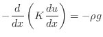
whose stiffness varies from end to end. The result is the equation
, representing a rope (or spring)
whose stiffness varies from end to end. The result is the equation
When  , this equation is called the ``Poisson equation'' and also describes
the distribution of heat in a solid bar, among other common physical problems.
, this equation is called the ``Poisson equation'' and also describes
the distribution of heat in a solid bar, among other common physical problems.
For the sake of definiteness, take
 and
and  , the left end of
height
, the left end of
height  at
at  , and the right end height of
  at
at  .
Thus, the system to be solved is
.
Thus, the system to be solved is
The ODE is linear. Linearity
implies good things such as the existence and uniqueness
of solutions.
Finite Difference Method for a BVP
The ``derivation'' presented above for the shape of the
rope is suggestive of a way to solve for the shape, called
the ``finite difference method.'' Assume that
we have divided the interval up into  equal intervals of
width
equal intervals of
width  determined by
  points. Denote the spatial
points
points. Denote the spatial
points  ,
,
 . Approximate the
value of
. Approximate the
value of  by
by  . Also approximate the Young's modulus
function as
. Also approximate the Young's modulus
function as
 .
.
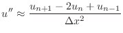
Now, consider the
 interval as if it were the differential
piece of rope mentioned in the derivation. Using the standard finite difference
approximation for a derivative, the slope of the rope at the left of
the
interval could be approximated as
interval as if it were the differential
piece of rope mentioned in the derivation. Using the standard finite difference
approximation for a derivative, the slope of the rope at the left of
the
interval could be approximated as
 and the slope on the right of the
interval could be
approximated as
and the slope on the right of the
interval could be
approximated as
 . The difference between
these is an approximation of the second derivative
. The difference between
these is an approximation of the second derivative
Along similar lines, approximate the first derivative as
Both approximations (of  and
and  ) have the same
Taylor-series (truncation) error of
) have the same
Taylor-series (truncation) error of
 .
.
Put all these together into (1) to get
and, as above,
and
.
We can associate this equation with the solution value at
,
except for  and
and  (do you see why?). Conveniently, those
are the points at which we have boundary conditions specified.
(do you see why?). Conveniently, those
are the points at which we have boundary conditions specified.
In particular, let us look at approximating our rope BVP at 6
points. We set up the ODE at points 1, 2, 3, and 4, and associate the
boundary conditions with the
and  solution values. Note
that
solution values. Note
that
 . I also
multiplied through by
. I also
multiplied through by
 to make things look nicer:
Actually, in Equation (2), the quantities  and
and  are not really variables, being fixed by the boundary conditions. Hence
the only variables are
are not really variables, being fixed by the boundary conditions. Hence
the only variables are  ,
,  ,
,  and
and  . The system can
be rewritten as
. The system can
be rewritten as
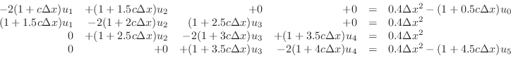
and this system has been formatted to suggest the matrix equation
![$\displaystyle \left[\begin{array}{rrrr} -2(1+c\Delta x)&+(1+1.5c\Delta x)&+0&+0...
...Delta x^2 0.4\Delta x^2 0.4\Delta x^2-(1+4.5c\Delta x)u_5\end{array}\right]$](img70.png) |
(3) |
By discretizing the differential equations we have created a set of
linear algebraic equations that have the symbolic form  .
To set up and solve the equations
(3) in Matlab, we could type:
.
To set up and solve the equations
(3) in Matlab, we could type:
N = 4;
C = 0.05;
RHOG = 0.4;
% N interior mesh points, N+1 intervals
dx = 5.0 / ( N + 1 );
x = dx * (0:N+1);
A = [ -2*(1+C*dx)    +(1+1.5*C*dx)        0             0;
      +(1+1.5*C*dx)  -2*(1+2*C*dx)  +(1+2.5*C*dx)       0;
            0        +(1+2.5*C*dx)  -2*(1+3*C*dx)  (1+3.5*C*dx);
            0              0        +(1+3.5*C*dx) -2*(1+4*C*dx) ];
ULeft=1;
URight=1.5;
b = [ RHOG*dx^2-(1+0.5*C*dx)*ULeft
      RHOG*dx^2
      RHOG*dx^2
      RHOG*dx^2-(1+4.5*C*dx)*URight];
U = A \ b;
U = [ULeft; U; URight]
Make sure you understand the first and last components in b.
You should recall that the backslash notation
is shorthand for saying U=inv(A)*b
but tells Matlab to solve the equation A*U=b
without actually forming the inverse of A.
Remark: The vector x is a row vector and the
vector U is a column vector! This is the convention that
has been followed for the _ode.m files and will be
followed throughout these labs.
-
- Exercise 1:
In this exercise, you will be using the above code to solve the rope
BVP. You will also be exhaustively checking that the code is correct.
- Copy the above code and paste it into a script m-file named
exer1a.m.
Execute exer1a to find a solution of Equation (3).
Please include the printed values of U as part of the lab summary.
- Verify that the values of U and b that
you found satisfy at least one of the middle four equations in (2).
To do this, write a script m-file named exer1b.m and plug
the values of
 ,
,
,
,
 into your chosen
equation. Show the result is essentially zero.
into your chosen
equation. Show the result is essentially zero.
Be careful! Lower-case
is upper-case C,
is dx and
 is U(1:6)
in exer1a.
is U(1:6)
in exer1a.
- Direct substitution into (3) shows that the
function
 would be a solution if
  and
and  .
As a second verification step, make a copy of exer1a.m
called exer1c.m with rhog=0 and URight=1
and check that the discrete solution is (exactly or to roundoff) correct.
.
As a second verification step, make a copy of exer1a.m
called exer1c.m with rhog=0 and URight=1
and check that the discrete solution is (exactly or to roundoff) correct.
- Direct substitution into (3) shows that the
function
 would be a solution if
  ,
,  and
and  .
As a third verification step, make a copy of exer1a.m
called exer1d.m with rhog=C and and with
boundary values ULeft and URight chosen to match
the solution you are testing.
Check that the discrete solution is (exactly or to roundoff) correct.
.
As a third verification step, make a copy of exer1a.m
called exer1d.m with rhog=C and and with
boundary values ULeft and URight chosen to match
the solution you are testing.
Check that the discrete solution is (exactly or to roundoff) correct.
- Direct substitution into (3) shows that the
function
 would be a solution if
 ,
,  and
and  .
As a fourth verification step, make a copy of exer1a.m
called exer1e.m with constant rhog, which
is used four times, replaced by the four values of the
vector 2+4*c*x(2:5)' and with
boundary values chosen to agree with
and check that the discrete solution is (exactly or to roundoff) correct.
.
As a fourth verification step, make a copy of exer1a.m
called exer1e.m with constant rhog, which
is used four times, replaced by the four values of the
vector 2+4*c*x(2:5)' and with
boundary values chosen to agree with
and check that the discrete solution is (exactly or to roundoff) correct.
- Now that you are confident that the code is correct, use
exer1a.m to solve the unmodified BVP (3).
Plot U versus x. It should appear roughly parabolic,
like a rope hanging from its ends, and pass through
 and
and  on its ends. Please include this plot with your summary.
Remark: The exact solutions  ,
,  , and
, and  can be used as exact discrete solutions and verification tests
only when the approximation expressions for first and second
derivatives are sufficiently accurate. Because the mesh is uniform,
the approximate expressions used here for the derivatives yield
the same values as using the usual continuous expressions so long as
can be used as exact discrete solutions and verification tests
only when the approximation expressions for first and second
derivatives are sufficiently accurate. Because the mesh is uniform,
the approximate expressions used here for the derivatives yield
the same values as using the usual continuous expressions so long as
 is a quadratic (or lower) polynomial, so there is no truncation
error and solutions are correct to roundoff.
is a quadratic (or lower) polynomial, so there is no truncation
error and solutions are correct to roundoff.
The purpose of the previous exercise is to verify that you have copied
the code correctly and to illustrate the powerful verification strategy
of checking against known exact discrete solutions.
You should always use a small, simple problem
to verify code by comparison with hand calculations. If possible,
you should also compare results with theoretical results and with
results achieved using a different method. In the next
exercise you will be modifying the above code to handle the
case of large N and solving a slightly more realistic problem.
Of course, you don't want to bother typing in the matrix
A if N is
100 or more, so you will be writing Matlab code to do it.
-
- Exercise 2:
- Make a copy of the script m-file exer1a.m and change it into
a function m-file called rope_bvp.m with the signature
function [x,U] = rope_bvp(N)
% [x,U] = rope_bvp(N)
% comments

% your name and the date
- Add comments after the signature line and modify the matrix
(A) and right side vector (b) generation statements
to be valid for arbitrary values of N. Make sure that the
vector U is a column vector. (You should also
eliminate the line N = 4.) Hint: You can use the
zeros(N,N) statement to generate an N-by-N
matrix of all zeros for A and then fill in the non-zero
values. You can use the command ones(N,1) to construct a column
vector of length N containing all ones.
- Check your work by running rope_bvp for N=4
and confirming that you get the same values of U as from
exer1a.m. One easy way to do this is to first run
exer1a, then use the command [x1,U1]=rope_bvp(4)
and check that U-U1 is the zero vector.
Debugging: If the results are not correct, print the matrix
A from rope_bvp and check it against the matrix
A from exer1a. Do the same for the vectors b.
Fix any mistakes before continuing.
- You may still have mistakes in the treatment of N. To
be sure of your code, make a copy of rope_bvp.m and
modify it to get the constant solution
as you did for
exer1c.m above. Check your results for N=4.
Fix any mistakes before continuing.
If you cannot find your mistakes
by checking your code, re-do Equations (2) for  and check the terms against your code, one term at a time.
- As a second test, make a copy of rope_bvp.m and
modify it to get the linear solution
as you did for
exer1d.m above. Check your results for N=4.
Fix any mistakes before continuing.
If you cannot find your mistakes
by checking your code, re-do Equations (2) for
and check the terms against your code, one term at a time.
- As a third test, make a copy of rope_bvp.m and
modify it to get the quadratic solution
as you did for
exer1d.m above. Check your results for N=4.
Fix any mistakes before continuing.
If you cannot find your mistakes
by checking your code, re-do Equations (2) for
and check the terms against your code, one term at a time.
- Now we are ready to solve the big problem! Use N=119
so that there are 119 unknowns U(1:119).
Call the new solution [x2,U2], and plot U2 versus x2.
Re-run exer1a to get U and x, and
plot U versus x as circles (plot(x,U,'o') on
the same frame (hold
on) and send the single frame with both plots to me with the
summary. To help in grading, please include the value of U(50)
in your summary.
Remark: You may wonder why the four-point mesh solution
and the 119-point mesh solution seem to agree at the four common points.
This behavior is highly unusual. It happens because the
solution of the differential equation is almost quadratic and the
difference scheme exactly reproduces quadratic functions. For larger
values of
, the solution looks less like a quadratic, and the
solution for  agrees less well with the solution for
  .
Try it, if you wish.
.
Try it, if you wish.
Finite element method
In the previous section, you saw an example of the finite difference
method of discretizing a boundary value problem. This method is based
on a finite difference expression for the derivatives that appear in
the equation itself. The finite difference method results in a
list of values that approximate the true solution at the set of mesh
points. Approximate values between the mesh points might be generated
using interpolation ideas, but the method itself does not depend on
any such interpolation. The reason that
was chosen for comparison
with
in the previous exercise is because the four
values in the
case appear among the  -values in the
case.
-values in the
case.
An alternative approach, called the ``finite element method'' (FEM) is based on
approximating the unknown as a sum of simple ``shape functions'' defined
over the mesh intervals. Since the finite element solution is actually
a function, it is defined over the same spatial interval as the true
solution and much of the machinery of functional analysis is available
for proving facts about the method and solutions that arise. As a
consequence, the FEM occupies a large part of the
mathematics literature.
You can find the FEM discussed
in Quarteroni, Sacco, and Saleri, Sections 12.4 and 12.5.
In this section, you will see the FEM applied to a particular
boundary value problem. The problem is somewhat simpler
than the clothesline problem discussed above, but contains the
same essential features. Consider the equation
 |
(4) |
defined for
in the interval ![$ [0,1]$](img97.png) , for
, for  a given function,
and with boundary values
a given function,
and with boundary values
 |
(5) |
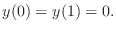
While the finite difference method attacks (4) directly,
the FEM starts from the so-called ``weak'' form of the equation. This
form can be constructed from (4) by multiplying through by a
function  , assumed to satisfy the same boundary conditions
(5), and integrating some terms by parts. In this case,
the weak form is given by
, assumed to satisfy the same boundary conditions
(5), and integrating some terms by parts. In this case,
the weak form is given by
Since
satisfies (5), the bracketed term
drops out and the result is
 |
(6) |
Remark: In this case, only the first term has been
integrated by parts. Some authors might also integrate the second
term by parts. Doing so would not change the following discussion very
much.
To approximate the function  , choose an odd integer
and a
set of functions
, choose an odd integer
and a
set of functions  for
for
 , defined on the interval
, that form a basis
of some reasonable approximating function space. For most finite element
constructions, these functions satisfy the following characteristics:
, defined on the interval
, that form a basis
of some reasonable approximating function space. For most finite element
constructions, these functions satisfy the following characteristics:
- They are continuous and piecewise polynomials.
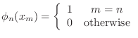
- Each of the functions takes the value 1 at a single mesh node
and zero at all other mesh nodes.
In this exercise, the functions will be piecewise quadratic polynomials
and the mesh nodes are given by
dividing the interval into
subintervals, each of length  ,
so that a sequence of spatial points is given by
,
so that a sequence of spatial points is given by  for
for
 (
( and
and  ). The quadratic
Lagrange functions are defined in the following way
(see Quarteroni, Sacco, Saleri, p. 562).
). The quadratic
Lagrange functions are defined in the following way
(see Quarteroni, Sacco, Saleri, p. 562).
This collection of functions is known to form a basis for a function
space that includes all constant, linear, and quadratic functions on
and it has good approximation properties. It is also true
that each of the functions
, for
 satisfies
the boundary conditions (5).
satisfies
the boundary conditions (5).
Assume that an approximate solution to (6) can be written
as
 |
(9) |
for (as yet unknown) constants  .
Plugging (9) into (6)
and choosing
.
Plugging (9) into (6)
and choosing
 yields
equations of the form
yields
equations of the form
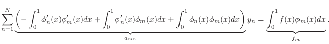 |
(10) |
Regarding the values
as the components of a (column) vector
 , the values
  as the components of a matrix
 , and the values
  as the components of a (column)
vector
as the components of a (column)
vector
 , then (10) can be written as the
matrix equation
, then (10) can be written as the
matrix equation
 |
(11) |
Solving the matrix equation (11) completes construction
of the approximate solution (9).
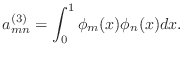
In the following exercises, you will write Matlab functions to construct
the basis functions
in (7) and (8),
to evaluate the matrix elements
and vector components
 in (10), and solve the matrix equation
(11).
in (10), and solve the matrix equation
(11).
Remark: When the FEM is programmed, the integrals in
(11) are typically performed element-by-element.
This is particularly important in multidimensional cases. Nontheless,
we will be using a conceptually simpler approach to the integrations.
-
- Exercise 3: In this exercise, you will construct the Lagrange quadratic basis functions.
The values
 used in (7) and (8) will be
evaluated as
used in (7) and (8) will be
evaluated as  , where
. The expression
, where
. The expression  is valid
even when
is valid
even when  , although Matlab does not allow subscripts equal to zero.
In the Matlab functions below, you should regard the variable x
as a scalar value, not a vector. Attempting to write vector
(componentwise) code only complicates matters here.
- Write a Matlab function m-file for
by completing the
following outline
function z=phi(n,h,x)
% z=phi(n,h,x)
% Lagrange quadratic basis functions

% your name and the date

if numel(x) > 1
  error('x is a scalar, not a vector, in phi.m');
end

if mod(n,2)==0  % n is even

  if (n-2)*h < x & x <= n*h
    z= ??? code implementing first part of (7) ???
  elseif n*h < x & x <= (n+2)*h
    z= ??? code implementing second part of (7) ???
  else
    z=0;
  end

else  % n is odd

  ??? code implementing (8) ???

end
- Plot some of your functions using the following code
N=7;
h=1/(N+1);
x=linspace(0,1,97);
mesh=linspace(0,1,N+2);
for k=1:numel(x)
  y3(k)=phi(3,h,x(k));
  y4(k)=phi(4,h,x(k));
end
plot(x,y3,'b')
hold on
plot(x,y4,'r')
plot(mesh,zeros(size(mesh)),'*')
hold off
You should observe that each  takes the value 1 at a single
mesh node (x(k), indicated with an asterisk), takes the value
zero at all other mesh nodes, is continuous, and is parabolic or zero
between any two mesh nodes. Please include this plot
with your summary file.
takes the value 1 at a single
mesh node (x(k), indicated with an asterisk), takes the value
zero at all other mesh nodes, is continuous, and is parabolic or zero
between any two mesh nodes. Please include this plot
with your summary file.
- Examine the definitions (7) and (8) and
show that
is a continuous function by showing that
the pieces match up at
 ,
,  , and
, and  for even
  and at
  and
and  for odd
. (You don't need Matlab
to do this.) Similarly, show that
for odd
. (You don't need Matlab
to do this.) Similarly, show that
- Write a Matlab function m-file similar to phi.m
for the derivative
 . Differentiate (7) and (8)
by hand to find
. Differentiate (7) and (8)
by hand to find
 and use your
formulæ for the function phip.m with signature
and use your
formulæ for the function phip.m with signature
function z=phip(n,h,x)
% z=phip(n,h,x)
% derivative of Lagrange quadratic basis functions

% your name and the date
- For the case N=7, plot
 and
and
 (multiply
by
(multiply
by  to get a better scaling) on the
same plot. Examine the plot carefully and convince yourself that
to get a better scaling) on the
same plot. Examine the plot carefully and convince yourself that
 appears to be the derivative of
  .
.
- Similarly, plot
 and
and  . Examine both cases from
(7).
. Examine both cases from
(7).
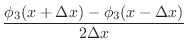
- For the case N=7 and the point
 , use the finite difference
expression
, use the finite difference
expression
with
 to estimate
 . Does it agree up to
roundoff with the result from phip? Similarly for
.
. Does it agree up to
roundoff with the result from phip? Similarly for
.
In the following three exercises, you will write m-files to construct and
verify the three pieces of the matrix A in (10). Following
that, you will construct the full matrix A and solve for the finite element
solution of the given problem (4).
-
- Exercise 4: In this exercise, you will generate the first part of the matrix
,
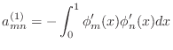 |
(12) |
You will be using many of the mathematical facts about this quantity in
order to check that your code is correct.
In order to do the integrations, you will be using code that I give you
that provides a uniform way to do the required integrations.
- Download a copy of a special integration function
gaussquad.m.
This code takes the names of two functions
(such as 'phi' or 'phip') along with their appropriate
subscripts and the value of the mesh spacing h and integrates
the resulting product over the interval [a,b]. Its signature is
function q=gaussquad(f1,k1,f2,k2,h,a,b)
This gaussquad function will provide the exact value,
not merely an approximate value, of the
integral for the cases considered in this lab: piecewise low degree
polynomials.
- Choose N=7 and h=1/(N+1), and write an m-file named
exer4.m to
compute the matrix values
 in (12). Call the resulting
matrix A1. Do not overlook the fact that the basis function
derivatives appear in (12), not the basis functions themselves, and
there is that pesky minus sign in front of the integral. Please
include the values of A1 in your summary file.
in (12). Call the resulting
matrix A1. Do not overlook the fact that the basis function
derivatives appear in (12), not the basis functions themselves, and
there is that pesky minus sign in front of the integral. Please
include the values of A1 in your summary file.
Remark 0: The following two remarks concern program efficiency.
Real programs intended to solve large problems should be concerned with
efficiency, but the first time you write a program you should strive
for simplicity and clarity. It is easier to make a correct program
run fast than it is to make a fast program run correctly.
Remark 1: The support of
is contained in the
interval
![$ [(n-2)h,(n+2)h]$](img153.png) . You could use this fact to shrink
your integration limits and improve the efficiency of the integration,
but it is not required.
. You could use this fact to shrink
your integration limits and improve the efficiency of the integration,
but it is not required.
Remark 2: Because the support of
and of  do not intersect when
 , you can take advantage of this fact to
avoid computing components
that must be zero, but it is
not required.
, you can take advantage of this fact to
avoid computing components
that must be zero, but it is
not required.
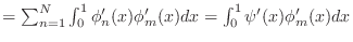
- (12) indicates that the matrix A1 is symmetric. Check
that your computation is symmetric by showing that
norm(A1-A1','fro')
is zero or roundoff. Add this code to exer4.m.
- For the case N=7 and h=1/(N+1), add code to
exer4.m to
compute the function
 for the 97
values x=linspace(0,1,97) and plot it. You should observe that
it is equal to 1 except near the endpoints of the interval. As a consequence,
it has zero derivative, except near the endpoints of the interval. Please
include the plot with your summary.
for the 97
values x=linspace(0,1,97) and plot it. You should observe that
it is equal to 1 except near the endpoints of the interval. As a consequence,
it has zero derivative, except near the endpoints of the interval. Please
include the plot with your summary.
- Since A1*ones(N,1)
 , and you just saw that
  is zero
except for
is zero
except for
 and
and
 ,
verify the zeros in positions
,
verify the zeros in positions  .
.
- Noting that
 , you
should be able to see why the following code
, you
should be able to see why the following code
N=7;
h=1/(N+1);
v=(1:N)'*h; % v=x
A1*v
should yield a vector that is zero except in the positions  .
Add this code to exer4.m and verify that it does.
.
Add this code to exer4.m and verify that it does.
- Recall that the BVP
 with
with
 has solution
 . You can solve this BVP using FEM.
Write a Matlab function m-file with the signature
. You can solve this BVP using FEM.
Write a Matlab function m-file with the signature
function z=rhs4(n,h,x)
% z=rhs4(n,h,x)

% your name and the date
to compute the constant function equal to (-2) everywhere. (This is
an almost trivial exercise. It is needed so that gaussquad.m
can be used.) Add code to exer4.m to use
the gaussquad.m function to compute the vector components
 and call the resulting vector
RHS4. Since the quadratic function
satisfies the
boundary conditions, it can be written exactly as a combination
of the
and call the resulting vector
RHS4. Since the quadratic function
satisfies the
boundary conditions, it can be written exactly as a combination
of the  ! Hence, the following code should yield the zero vector.
N=7;
h=1/(N+1);
xx=(1:N)'*h;   % the variable x has already been used.
v=xx.*(1-xx);
v-A1\RHS4  % should be zero
Add this code to exer4.m.
Please include the values of RHS4 in your summary.
The tests in exer4.m construct and test the matrix A1,
so you should now be reasonably sure that A1 is correct.
In the following exercise, you will construct and test A3.
In the subsequent exercise, you will construct and test
A2 so that you have all of the matrix A.
-
- Exercise 5:
- Start writing an m-file named exer5.m similar to
exer4.m but for the terms
Call the resulting matrix A3. Include this matrix
in your summary.
Warning: If you copy code from A1 for A3,
don't forget that A1 has a minus sign in it from the integration
by parts but that A3 does not.
- Add code to check that A3 is symmetric.
- Note that the boundary value problem
 |
(13) |
with
has the exact solution  , and this quadratic
function can be expressed exactly as a sum of the
.
, and this quadratic
function can be expressed exactly as a sum of the
.
- Write a Matlab function m-file rhs2.m with signature
function z=rhs5(k,h,x)
% z=rhs5(k,h,x)

% your name and the date
to compute the function
 . Add code to exer5.m
to use rhs5.m and gaussquad.m
to compute the (column) vector
. Add code to exer5.m
to use rhs5.m and gaussquad.m
to compute the (column) vector
 , and call
the resulting vector RHS5. Include these values in your summary
, and call
the resulting vector RHS5. Include these values in your summary
- The matrix A1 was computed by exer4.m, and
A2 and RHS5 are computed by exer5.m. Add
code to exer5.m to
solve the matrix equation (A1+A3)*Y=RHS5. You have just solved
(13), and your solution should equal
 at each of the nodes
exactly, with only roundoff errors.
Add code to exer5.m to check that this is true.
If it is not true, there is a mistake somewhere. Fix it before continuing.
at each of the nodes
exactly, with only roundoff errors.
Add code to exer5.m to check that this is true.
If it is not true, there is a mistake somewhere. Fix it before continuing.
-
- Exercise 6:
- Write another m-file named exer6.m to compute the terms
 |
(14) |
Call this matrix A2.
Include this matrix in your summary.
- Integrating (14) by parts and applying the
boundary conditions shows that the matrix A2 is skew-symmetric
(i.e., A2'=-A2. Add code to exer6.m
to confirm this is true.
- Note that
adding the terms A1, A2 and A3 together
generates the matrix A.
- Note that boundary value problem
 |
(15) |
with boundary values
has exact solution
.
- Write a Matlab function m-file rhs6.m with signature
function z=rhs6(k,h,x)
% z=rhs6(k,h,x)

% your name and the date
to compute the function
 .
Add code to exer6.m
to compute the (column) vector
.
Add code to exer6.m
to compute the (column) vector
 , and call
the resulting vector RHS6.
, and call
the resulting vector RHS6.
- Solve the matrix equation A*Y=RHS6. You have just solved
(15), and your solution should equal
exactly, with only roundoff errors.
Remark: Writing test scripts like exer4.m,
exer5.m and exer6.m allows you to re-test your work
at any time. This strategem helps you maintain confidence in your code
and also allows you to propose and test modifications easily.
-
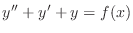
- Exercise 7: The boundary value problem
with boundary values
has exact solution
 , with
 .
.
- Write a function m-file exact7.m to evaluate the
above exact solution.
- Write a function m-file rhs7.m to evaluate the right side
function
 .
.
- Write a function m-file solve7.m with signature
function [x,Y]=solve7(N)
% [x,Y]=solve7(N)
%    ... more comments ...

% your name and the date
that performs the following tasks:
- Compute the finite element matrix A
- Compute the right side vector RHS7
- Solve the system A*Y=RHS7 for Y
- Compute the spatial coordinate vector (1:N)'*h
- Fill in the following table and estimate the rate of convergence
of this method. Measure the error as the maximum absolute value
of the difference between the calculated and true solutions at the
nodes
, and
take the ratio as the error(h) divided by error(h/2).
  N    h        error      ratio
  7  1.2500e-1  ________  ________
 15  6.2500e-2  ________  ________
 31  3.1250e-2  ________  ________
 61  1.6129e-2  ________  ________
121  8.1967e-3  ________
Remark: The rate of convergence appears higher than
expected from theory. This rate is an artifact of the way the error
is computed. To do it properly, one needs to compute  integral
errors that involve more than just the node points. Convergence at
the node points is one higher order than expected, a feature called
``superconvergence.''
integral
errors that involve more than just the node points. Convergence at
the node points is one higher order than expected, a feature called
``superconvergence.''
Burgers' Equation
A partial differential equation (PDE) involves
derivatives of a function
which depends on more than one
independent variable. One interesting PDE is the one-dimensional
Burgers' equation, which is a one-dimensional nonlinear equation
whose nonlinear term is similar to the one in the Navier-Stokes equations
of fluid flow. In this case, the variable will be called
and it
is a function of space (
) and time ( ),
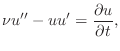
),  . The variable
is called ``velocity'' in the Navier-Stokes equations.
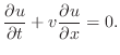
Burgers' equation on the spatial interval
can be written as
. The variable
is called ``velocity'' in the Navier-Stokes equations.
Burgers' equation on the spatial interval
can be written as
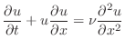 |
(16) |
where  is a constant. Boundary conditions can be taken as
 and
and  , both for all time. Two space boundary conditions
are necessary because the equation is second-order in space.
Since the equation is first-order in time, only one intitial condition
is needed.
, both for all time. Two space boundary conditions
are necessary because the equation is second-order in space.
Since the equation is first-order in time, only one intitial condition
is needed.
To get an idea of what the solution to Burgers' equation might look like,
first imagine that  and also that the coefficient
  is a constant,
so that the equation becomes the wave equation
is a constant,
so that the equation becomes the wave equation
If  , this equation represents a right-going wave that moves without
changing shape. To see this, note that for any given function of one
variable,
, this equation represents a right-going wave that moves without
changing shape. To see this, note that for any given function of one
variable,  ,
,  is a solution of the wave equation. Changing
to a small, positive number means that the wave propagates as before,
but slowly spreads and decays to zero. Finally, since the coefficient
is a solution of the wave equation. Changing
to a small, positive number means that the wave propagates as before,
but slowly spreads and decays to zero. Finally, since the coefficient  is
not constant, the wave propagates faster where
is larger and
slower where
is smaller. Thus a wave that is larger to the left and
smaller to the right will steepen as it propagates to the right.
is
not constant, the wave propagates faster where
is larger and
slower where
is smaller. Thus a wave that is larger to the left and
smaller to the right will steepen as it propagates to the right.
The Method of Lines
Look at (16) and pretend, just for a moment, that
time is frozen. The equation suddenly starts looking like the
boundary value problem (1) that we solved before,
only with a extra
term on the left and with
 replacing the right
side. This observation is the
basis for the ``method of lines,'' wherein the spatial
discretization is performed separately from the temporal. Consider
the function
replacing the right
side. This observation is the
basis for the ``method of lines,'' wherein the spatial
discretization is performed separately from the temporal. Consider
the function  , but think of it as a
function of
first. The resulting BVP can be
written with primes denoting spatial differentiation so it
looks more like what we have been doing.
, but think of it as a
function of
first. The resulting BVP can be
written with primes denoting spatial differentiation so it
looks more like what we have been doing.
where we are focussing on the left side for the moment,
along with spatial boundary conditions
and 
We solved a BVP a lot like this one above. We broke the interval
into  subintervals and labelled the
 resulting points
 . Next, we
defined
. Next, we
defined  as being the approximate
solution at
. Keep in the back of you mind,
though, that
is really still a function of
,
as being the approximate
solution at
. Keep in the back of you mind,
though, that
is really still a function of
,
 . We will denote the vector of values
by
. We will denote the vector of values
by  , because we
have already used the unsubscripted
to denote the continuous
solution. Keep in mind that
, because we
have already used the unsubscripted
to denote the continuous
solution. Keep in mind that  is a function of time. We will
use the same finite difference discretization as before for the term
is a function of time. We will
use the same finite difference discretization as before for the term 
 |
(17) |
and will choose a natural discretization for the first-order nonlinear term
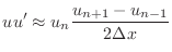 |
(18) |
(The truncation error of each of these forms is
.) The
resulting discrete equations become
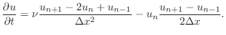 |
(19) |
But we remain on familiar ground: (19) is just a system of IVPs!
We know a bunch of different methods to solve it. It turns out that
the system is moderately stiff, and will become more stiff when N
is taken larger and larger. We will use backwards Euler to solve this
system. Recall that backwards Euler requires an m-file to evaluate
both the function
and its partial derivative (Jacobian)
 |
(20) |
In Matlab notation, the variable
will be a matrix whose
entries  approximate the values
  . In Matlab
notation, for the
. In Matlab
notation, for the
 time interval, U(:,k)
represents the (column vector of) values at the
locations x(:). The initial condition for U
should be a column vector whose values are specified at
the locations x(:).
time interval, U(:,k)
represents the (column vector of) values at the
locations x(:). The initial condition for U
should be a column vector whose values are specified at
the locations x(:).
-
- Exercise 8: In this exercise you will write, debug, and solve an m-file for the
solution of Burgers' equation in the form of (19) with
 and using N=500.
- Begin a function m-file called burgers_ode.m to construct the
spatial discretization of Burgers' equation and its gradient. The function
refers to the right side of (19).
Here is an outline:
function [F,D]=burgers_ode(t,U)
% [F,D]=burgers_ode(t,U)
% compute the right side of the time-dependent ODE arising from
% a method of lines reduction of Burgers' equation
% and its derivative, D.
% Boundary conditions are fixed =0 at the
% endpoints x=0 and x=1.
% A fixed number of spatial points (=N) is used.
% The variable t is not used, but is kept as a place holder.
% U is the vector of the approximate solution at all spatial points
% output F is the time derivative of U (column vector)
% output D is the Jacobian matrix of
%   partial derivatives of F with respect to U

% spatial intervals
N=500;
NU=0.001;
dx=1/(N+1);
ULeft=1;  % left boundary value
URight=0; % right boundary value

F=zeros(N,1);  % force F to be a column vector
D=zeros(N,N); % matrix of partial derivatives

% construct F and D in a loop
for n=1:N
  if n==1  % left boundary
     F(n)  = ??? Function, left endpoint ???
     D(?,?)= ??? Derivative, left endpoint ???
  elseif n<N  % interior of interval
     F(n)  = ??? Function, interior points ???
     D(?,?)= ??? Derivative, interior points ???
  else % right boundary
     F(n)  = ??? Function, right endpoint???
     D(?,?)= ??? Derivative, right endpoint???
  end
end
- It is easiest to treat the interior points
(the case n<N) first. Replace the line
F(n)= ??? Function, interior points ???
with the discretization for F(n) given in (19).
- Replace the line
D(?,?)= ??? Derivative, interior points ???
with the values D(n,n), D(n,n+1), and D(n,n-1)
according to the formula that was given above in (20)
and is repeated here.
 |
(21) |
The variable  will take on the three values n, n+1,
and n-1. To do, for example, D(n,n+1), write out
the expression for F(n) and differentiate it with respect
to U(n+1). Remark: It is easy to see from the formula that
will take on the three values n, n+1,
and n-1. To do, for example, D(n,n+1), write out
the expression for F(n) and differentiate it with respect
to U(n+1). Remark: It is easy to see from the formula that
 for
for  or
or  .
.
- When n=1, the variable corresponding with n-1
is the left boundary value ULeft. With this in mind,
replace the lines
     F(n)  = ??? Function, left endpoint ???
     D(?,?)= ??? Derivative, left endpoint ???
with the expressions for F(n), D(n,n) and D(n,n+1).
- When n=N, the variable corresponding with n+1
is the right boundary value URight. With this in mind,
replace the lines
     F(n)  = ??? Function, right endpoint???
     D(?,?)= ??? Derivative, right endpoint???
with the expressions for F(n), D(n,n) and D(n,n-1).
- The spatial values represent a uniform mesh
N=500;  % must agree with value inside burgers_ode.m
x=linspace(0,1,N+2);
x=x(2:N+1);
and we will assume an initial velocity distribution that looks like
a shallowly sloped wave.
UInit=((1-x).^3)';
- Test your version of burgers_ode.m by calling it
with UInit (the value of t does not matter) and comparing
the result with the following values:
                results burgers_ode(0,UInit)
  n       F(n)      D(n-1,n)       D(n,n)      D(n+1,n)
  1 2.9761711475                -499.01396011  498.51296011
  2 2.9465759259    1.99800798  -499.02590030  497.02789232
250 0.0976958603  219.12262501  -501.24899902  282.12637400
499 2.395210e-05  251.00094622  -502.00194821  251.00100199
500 1.197605e-05  251.00098406  -502.00198406
- Retrieve your copies of back_euler.m and
newton4euler.m, or download my copies of
back_euler.m
and
newton4euler.m.
- Use back_euler to
solve Burgers' equation starting from UInit.
You should use 100 steps from time t=0 to time t=1.
[t,U]=back_euler('burgers_ode',[0,1],UInit,100);
The solution should converge at each step. If you get the
``failed to converge'' message, your derivative (D)
is probably wrong. To help with grading, please include the value
of U(200,50) in your summary.
- Recall that the columns of U represent velocities
at different places all at the same time and rows of
U represent velocities at different times all
at the same place.
To see a snapshot of the solution at timestep k, use the
command
plot(x, U(:,k) )
where x is the value assigned above.
Please include this plot for the choice k=50 with your summary.
- You can see a ``flicker picture'' of the evolution
with the following steps
plot(x,U(:,1))
axis([0,1,0,1.5])
for k=2:100
  pause(0.1);
  plot(x,U(:,k));
  axis([0,1,0,1.5])
end
You should be able to see the ``wave'' steepen as it moves to the right.
Please include the final frame of this sequence with your summary.
Remark: The boundary condition is inappropriate for the case
that the ``wave'' actually reaches the right boundary, and the solution
will fail if the time interval is long enough for the wave to reach
 .
.
Extra Credit: Shooting Methods (8 points)
Shooting methods solve a BVP by reformulating it as an IVP, using initial
values as parameters. The BVP is solved by finding the parameters that
reproduces the desired boundary values. For this exercise, we return
to considering the BVP of a hanging rope.
Taking as our example the rope BVP (1),
how much violence do we have to do to it
in order to make it look like an IVP? Well, we expect to have two
conditions at the left point and none at the right point. So let's
temporarily consider the related problem, where we have made up an
extra boundary condition at our initial value of
:
The following exercise attacks this system using a method
called ``shooting.'' The strategy behind this method is the following.
- For each value of
 , we can solve this problem, and get a
numerical solution at a sequence of points up to the right endpoint.
, we can solve this problem, and get a
numerical solution at a sequence of points up to the right endpoint.
- Since every value of
determines a (numerical) solution
 , we can regard the
difference between the value we got, and the value we want, as a
function
, we can regard the
difference between the value we got, and the value we want, as a
function
 . (Where we write
,
but we should really write something like
. (Where we write
,
but we should really write something like
 , to emphasize that the
solution depends on the parameter.)
, to emphasize that the
solution depends on the parameter.)
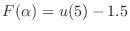
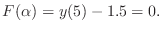
- The BVP solution we are looking
for has the property that
 . The Matlab function
fzero will be used to find
. The Matlab function
fzero will be used to find  .
.
As you know, the ODE (1) can be written as a system
of first order differential equations. This is done by
identifying  and
and  , yielding the system
For this exercise, you will be using built-in Matlab ODE
routines to solve the initial value problem that arises from a guessed
initial condition and then you will use the Matlab
function fzero to solve for the correct initial condition.
-
- Exercise 9:
- Write a function m-file named rope_ode.m with signature
function fValue=rope_ode(x,y)
% fValue=rope_ode(x,y) computes the
% rhs of the first-order system

% your name and the date
Note that since we plan to use ode45 there is no need
to add the Jacobian matrix to rope_ode.m!
This is a great convenience, but in
many cases you would have to provide a function for the Jacobian
or ode45 (or ode15s, etc.) might fail. In
that case, setting an option allows the Jacobian computation.
- Choose a provisional value
 and use the Matlab
function ode45 to solve the system (22) on the
interval [0,5]. What is the value of
and use the Matlab
function ode45 to solve the system (22) on the
interval [0,5]. What is the value of  ? Is it positive
or negative? (Be careful: which of the components of y
corresponds with
?)
? Is it positive
or negative? (Be careful: which of the components of y
corresponds with
?)
- By trial and error, find a second value of
for which
the value of
is of the opposite sign as for
.
The correct value of
lies between the two values you just
found.
- Write an m-file called rope_shoot.m
that accepts a value of alpha and evaluates
F(alpha), for the rope BVP. The file should have the signature
function F = rope_shoot ( alpha )
% F = rope_shoot ( alpha )
% comments

% your name and the date
and this code should do the following:
- Use the input value of alpha as the initial condition for
 ;
;
- Use ode45 to compute the solution [x,y] of
the IVP (22) defined by the
initial conditions, and the right hand side function rope_ode,
for
![$ x\in[0,5]$](img242.png) ;
;
- Return in the function value F the value of
.
For a given value of
, the function you just wrote will return
 . When
is just right, it will return 0.
. When
is just right, it will return 0.
- Test that rope_shoot returns the same value you obtained
above when alpha=0.
- Use the Matlab function fzero to find the value of
that makes
 fzero
requires two parameters, a function handle (
fzero
requires two parameters, a function handle (@) first and
second the vector [alpha1,alpha2]
of the two values of
that you just found
for which  has opposite signs. What is the value of
alpha you found?
has opposite signs. What is the value of
alpha you found?
- Plot the solution you found. Does the curve have a
height of 1 at
and a height of 1.5 at
?
You do not need to send me this plot.
- Return to your solution for N=119 in Exercise 2.
Use a finite difference expression for the derivative to
estimate the derivative of U2 at the left endpoint.
How does it compare with the value
you just computed?
Back to MATH2071 page.
kimwong
2019-02-08
![$\displaystyle -K\left.\frac{du}{dx}\right]_{\mbox{right}}+K\left.\frac{du}{dx}\right]_{\mbox{left}}
=- \rho g dx. $](img11.png)
![$\displaystyle -\int_0^1 y'(x)v'(x)dx + \left[\rule{0pt}{12pt}y'(x)v(x)\right]_0^1 +\int_0^1 y'(x)v(x)dx +\int_0^1y(x)v(x)dx=\int_0^1f(x)v(x)dx$](img101.png)
![\begin{displaymath}\left\{
\begin{array}{ll}
\frac{(x-x_{n-1})(x-x_{n-2})}{(x_n-...
...x \leq x_{n+2} [5pt]
0 & \text{ otherwise}
\end{array}\right.\end{displaymath}](img113.png)
![$\displaystyle \left\{\begin{array}{ll}
\frac{(x_{n+1}-x)(x-x_{n-1})}{(x_{n+1}-x...
...or } x_{n-1}\leq x\leq x_{n+1} [5pt]
0 & \text{ otherwise}
\end{array}\right.$](img114.png)