
| HPS 0410 | Einstein for Everyone |
Back to main course page
John
D. Norton
Department of History and Philosophy of Science
University of Pittsburgh
Background reading: J. P. Mc Evoy and O. Zarate, Introducing Stephen Hawking. Totem. pp. 46-105.
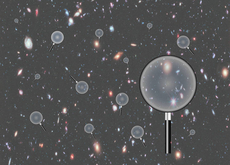
Which solutions of Einstein's gravitational field equations can accommodate a universe with a Hubble expansion? Or, more figuratively, which pages in Einstein's great book might belong to our universe?
| It may seem an overwhelming task to pore through the pages of Einstein's great book to find those that might be our universe. However it is not so. We need to pick just two properties of the spacetime to narrow down our choices to a family of spacetimes that form the basis of modern, relativistic cosmology. | The situation is not so different from someone trying to identify a small country in a huge atlas of the world. The atlas may be huge. But, if it is well made, one needs only a few key words and a good index to arrive rapidly at the page of interest. |
The two conditions are that the ordinary, three dimensional spaces of our cosmos are homogeneous and isotropic; and that space is filled uniformly with matter. They suffice to identify a class of solutions of Einstein's equations known as the Friedmann-Lemaitre-Robertson-Walker spacetimes.
Recall how we first built a spacetime many chapters ago. We took all of space at many instants of time and stacked these spaces up into a fourth, temporal dimension to generate spacetime.
| We will stack these spaces again to build the spacetimes of relativistic cosmology. When we first stacked these spaces to build a Minkowski spacetime of special relativity, we assumed tacitly with Einstein and Minkowski that space was Euclidean. No other possibility seemed reasonable when special relativity was born. Now we know better. The spaces we will stack up do not have to be Euclidean. We will leave open the possible geometries. | That a spacetime can be built up this way seems obvious and natural. However not all spacetimes can be built up this way. We have already seen one. A Goedel universe cannot be sliced up nicely into spaces that evolve into each other over time. Reversing the failure, we cannot build a Goedel spacetime by stacking up snapshots of space taken at different moments of time. |
What geometries can the spaces have? The observations of our cosmos tell us that, on the largest scale, space at any instant of time is homogeneous and isotropic. So we ask that the geometries of the spaces we stack up are homogeneous and isotropic . That means that, in each case, the geometry of the space is the same in every place (homogeneous) and is the same in all directions (isotropic).
| This condition that the cosmos is homogeneous and
isotropic on the largest scale is sometimes derived from the "cosmological
principle." In a standard form, that principle asserts that "... broadly speaking ... the universe presents the same aspect from every point except for local irregularities." Hermann Bondi, Cosmology. 2nd ed. Cambridge University Press, 1960 p. 11. This principle applies to everything in the cosmos. That "everything" includes the geometry. If then follows from the cosmological principle that the geometry of space is everywhere the same. It strikes me as a little dangerous to label a vaguely formulated, happenstance regularity as a "principle." We generally reserve that term for laws of nature or perhaps just for conditions that are not lightly challenged. Whether the universe is roughly homogeneous and isotropic is something that should be determined by observation. It should not be legislated in advance. We saw in the last chapter that those observations seem always to need to move to larger scales before we can secure homogenity and isotropy. |
The distinguishing of this loose idea of sameness
as a principle derives from the cosmological work
on E. A. Milne in the 1930s. He developed a cosmology in
which spatiotemporal relations were induced from considerations of
light signaling, somewhat like Einstein's analysis of special
relativity of 1905 and using analogous principles. His "cosmological
principle" was modeled on Einstein's principle of relativity and
read: "...if A and B are two equivalent particles of the system, then the description of the system by A (in terms of his clock-measures or associated coordinates) coincides with the description of the system by B in terms of B's clock-measures or associated coordinates." E. A. Milne, Relativity, Gravitation and World-Structure. Oxford: Clarendon Press,1935, p. 60. |
The condition that the space is homogeneous and isotropic restricts the geometry to three general possibilities. Such a space must have constant spatial curvature. We know from earlier that the three possibilities are:
| Spherical Positive curvature |
Flat, Euclidean Zero Curvature |
Hyperbolic Negative Curvature |
 |
 |
 |
A space of one of these three types will be the instantaneous snapshots that comprise the "now" of the cosmology.
 |
Caution! The spaces to which these three curvatures apply are just the ordinary, three-dimensional spaces produced when we take the instantaneous snapshots "now" of the whole spacetime. |
Each of these snapshots of space will be filled with a uniform matter distribution. Its composition is not fixed. However it is sufficient to distinguish two general types of matter to pick out the spacetimes.
The first type is ordinary matter, such as comprises planets and stars. We have seen that, on the larger scale, this matter is clustered into stars and then galaxies. On the largest scale, these galaxies fill space just as the molecules of air fill the space of a room. In both cases, if we work at a sufficiently large scale, we can ignore the granularity of individual molecules or galaxies. In both cases, matter behaves like a fluid. Sometimes, cosmologists label the galactic matter as "dust." To understand why, think of a dust so fine that flows like a fluid.

| At any cosmic moment, these particles of dust
fill space. Over time they trace out a bundle of
non-intersection, geodesic curves that fill the spacetime. Once
again, this idea has been elevated with the title of "postulate" or
"principle" as in "Weyl's Postulate." It
is named after the mathematician and relativist Hermann Weyl, who
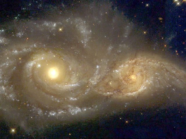
used the assumption in his work. Once again there is a danger in assigning the term "postulate" or "principle." It makes the assumption look like a fundamental law of nature, whereas it is clearly only an accident of our particular universe. Worse it is one that we have seen violated here and there through the observation of colliding galaxies. Here's an image from the NASA website of spiral galaxies NGC 2207 and IC 2163 colliding. |
The notion that there is a principle here seems to
have grown organically. It was implicit in much cosmological
theorizing in the 1920s and 1930s. R. C. Tolman, in his influential
1934 text, Relativity, Thermodynamics and Cosmology
(Oxford University Press), writes of "An alternative hypothesis
suggested by Weyl and ... by Robertson... the nebulae [galaxies] in
the actual universe are to be regarded as lying on a coherent pencil
of geodesics which diverge from a common point in the past." (pp.
356-57). On a haphazard survey, the earliest definite use of the term I found is Hermann Bondi's Cosmology. 2nd ed. Cambridge University Press, 1960, p. 100: ... Weyl's postulate: The particles of the substratum (representing the nebulae) lie in a space-time bundle of geodesics diverging from a point in the (finite or infinitely distant) past. Hermann Bondi and Thomas Gold, in an earlier paper, write of consequences of "Weyl's postulate," while not clearly specifying the postulate's content. (Monthly Notices of the Royal Astronomical Society, Vol. 108, no. 3 (1948) on p. 257.) A later textbook reproduces a derivative version of Bondi's wording: WEYL's postulate: The particles of the substratum (representing the nebulae) lie, in the space-time of the cosmos, on a bundle of geodesics diverging from a point in the (finite or infinite) past. R. K Pathria, Theory of Relativity. Pergamon, 1974, p. 266. |
.
The second type of matter is radiant matter. It is the type of matter Penzias and Wilson found to comprise the cosmic microwave background radiation. We need to make few assumptions about this second form of matter. All we need is that it is radiant and distributed homogeneously and isotropically in space.
We make no assumption about how much of the cosmic matter is ordinary "dust" and how much is radiant. How the relative proportions evolve will be recovered as a consequence of Einstein's theory. As we shall see below, our best efforts to infer back to the distribution lead us to unexpected results. There is a gap between the observed matter distribution and what the dynamics tells us. That gap is filled by a non-zero cosmological constant. It is often interpreted a form of matter, "dark energy."
Once we have specified these two conditions, we have narrowed the possibilities to the Friedmann-Lemaitre-Robertson--Walker spacetimes of modern relativistic cosmology. The remaining cosmic properties are now determined through them by Einstein's gravitational field equations.
| The most important property is that the spacetime is dynamic. That is, the spaces of the cosmology cannot remain unchanged. They are either expanding or contracting. As they do this, they carry matter with them. The first case of expansion is the one that interests us most, since it is what we observe in the expansion of the galaxies. | There are exceptions if we allow a non-zero cosmological constant Λ. We have seen earlier that a static Einstein universe comes about because the tendency of matter to coalesce gravitationally can be balanced exactly by a well-chosen value of Λ. What makes this case exceptional is that the value of Λ must be exactly right. If it is even slightly bigger or smaller than the balancing value, an expanding or contracting universe results. |
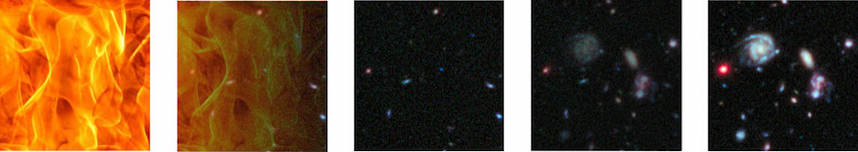
| There is a simple explanation that can be given for why radiation dilutes faster than ordinary "dust" matter. If we consider a tiny volume of the expanding space in an FLRW spacetime, it will behave classically to good approximation. The matter of dust will just be distributed over a larger volume of space, as the space expands. The energy of radiation will also be distributed over this same larger volume of space. If this effect were the only one present, then dust and radiant energy would dilute at the same rate. However there is a second effect concerning radiation. Radiation exerts a pressure and this pressure is exerted on the boundary of the little volume of space we are considering. That means that it does work on the boundary. Doing work means that it loses energy and this loss of energy results in the radiation diluting faster than dust. | In the early stages of this expansion, shortly after the big bang, most of the matter is in the form of extremely hot radiation. The universe is radiation dominated. As the expansion continues, the radiant matter cools and dilutes faster than the ordinary "dust" matter. In the later stages, such as our cosmos is in now, most of the matter is in the form of dust. Once we enter the ordinary matter dominated era, the matter starts to clump, drawn together by its mutual gravitational attraction. This clumping matter heats as it collapses together and nuclear fusion fires are ignited. What results are stars; and these stars in turn collect under mutual gravitational attractions into galaxies. |
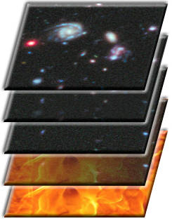
| We form the spacetime picture of this process by
stacking the snapshots of space. As space expands and matter is carried with it, the distance between the galaxies increases. The figure below shows the worldlines of the galaxies piercing through the growing spatial slices, the snapshots of space at different moments of time. The expansion affects the geometry of space as well. As time passes, space at one time expands and evolves into space at a later time. In the process, the curvature of space, if it has any, decreases. |
 |

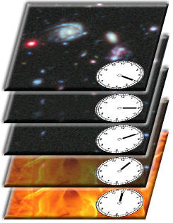 |
These spacetimes come equipped with a unique notion of cosmic time. It appears as the uniqueness of the slicing up of the spacetimes into ordinary three dimensional spaces. Cosmic time is measured by the proper time elapsed along the world lines of the galaxies. The cosmic epoch associated with each snapshot of space is given by the proper time elapsed after the big bang. In this sense, there is a cosmic notion of simultaneity and a natural clock ticking in the universe. |
These spacetimes differ from the Minkowski spacetime of special relativity. In a Minkowski spacetime, we are free to slice up the spacetime in many equivalent ways into ordinary, three-dimensional spaces. This was the geometric expression of the relativity of simultaneity. It derived directly from the equivalence of all inertial frames of reference and the fact that there is no absolute state of rest in special relativity.
| This feature is lost in the Friedmann-Lemaitre-Robertson-Walker spacetimes. There is now a unique way to slice up the spacetimes into ordinary, three-dimensional spaces. It is shown in the figures above. One might worry that this somehow contradicts special relativity. It does not. Special relativity is the theory that describes Minkowski spacetimes. The Friedmann-Lemaitre-Robertson-Walker spacetimes are not Minkowski spacetimes and will not conform to the requirements of special relativity. | There is an exception, described below: the de Sitter spacetime. |
On might still worry that this unique way of slicing up the spacetimes introduces something undesirable, perhaps akin to the absolute state of rest of the nineteenth century ether. That does not happen. The problem with the nineteenth century ether was that its absolute state of rest was unobservable. One inertial state of motion out of infinitely many, we were assured, corresponded to absolute rest. However no observation could tell us which was that special one. This aroused great suspicions for being in a state of absolute rest was a difference that made no difference.
There is no corresponding problem in these cosmological spacetimes. There is a unique state of rest and it is observable. It is the frame of reference in which cosmic matter is distributed uniformly. If we are at rest in that frame of reference, we will observe cosmic matter to be distributed uniformly around us. If we are moving relative to this cosmic rest frame, we will observe anisotropies. The situation is quite like what happens when we move through calm air. We know that we are moving through the air in a definite direction because we feel the pressure of the air on the leading side.
 |
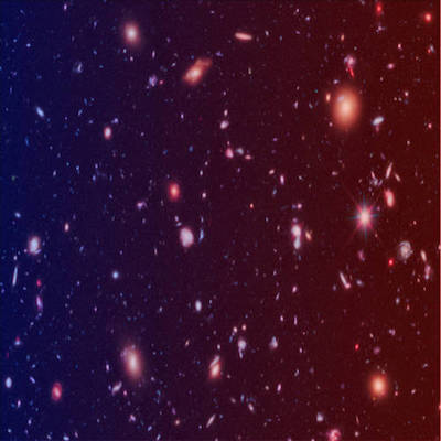 |
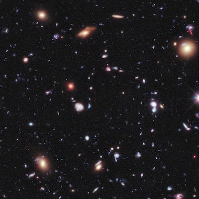
| In the cosmic rest frame, the galaxies are distributed uniformly through space. | If we move relative to the cosmic rest frame, the distribution of galaxies is compressed in the direction of motion. This is the familiar length contraction already seen in special relativity. The Doppler shift also produces an effect. Light arriving from the direction of our motion is blue shifted and light from the opposite direction is red shifted by the Doppler effect. The image above portrays the case of motion to the left. |
| As reported in Planck collaboration, "Planck 2018 results. I. Overview and the cosmological legacy of Planck," https://arxiv.org/abs/1807.06205 | As it happens, we are not precisely at rest
according to this cosmic frame. We are moving, slowly by cosmic
standards. A recent estimate puts the motion of our sun at roughly
at 370 kilometers per second towards
the constellation of Leo. We know this by measurements in the cosmic
background radiation. They reveal a slight Doppler shift
corresponding to this motion. This is the motion of our sun. The earth's motion will vary around this figure in the course of the earth's annual orbit around the sun. This orbital speed is almost 30 kilometers per second. A component of it must be added or subtracted to the motion of the sun to recover the earth's motion with respect to the cosmic background radiation. |
The most interesting feature of Friedmann-Lemaitre-Robertson-Walker spacetimes is what happens when we project the worldlines of the galaxies into the past. The galaxies get closer and closer. Eventually, they converge onto a state of infinite curvature and density. This is the initial state--the so-called "big bang," shown at the bottom of the figure above.
It is easy to misunderstand the nature of the big bang and the expansion of the universe.
The popular image called to mind by the name big bang is something like this. There is a huge empty space, with an infinitely dense nugget of matter containing all future matter of the universe. At the moment of the big bang, This nugget explodes. Fragments of this primeval nugget are scattered into space, progressively filling it with an expanding cloud of matter. This is NOT the modern big bang model.

Rather the expansion is the expansion of space itself. The most helpful picture is of the rubber surface of a balloon expanding. The galaxies are like dots drawn on the surface. They move as the rubber sheet stretches. The galaxies fly apart because space expands. At any instant, space is always full of matter; there is no island of fragments expanding into an empty space.

Here's how one fixed volume of space will look over the course of cosmic evolution.

If we now project back to the big bang, we project back to a time at which all matter and space were somehow compressed into a state of infinite density. Einstein's gravitational field equations tell us the matter density equals the summed spacetime curvature. So, if the matter density is infinite, the curvature of spacetime has become infinite as well.
That last statement cannot be literally correct. According to Einstein's general theory of relativity, spacetime at every event has definite curvature. If that curvature is everywhere infinite, we define no spacetime at all. If we try to imagine the time of the big bang itself as one of the times of the cosmology, we are saying that there is a time at which spacetime is not properly defined. So there can be no time in the cosmology corresponding to the big bang. We describe the big bang as a "singularity," a breakdown in the laws that govern space and time.

The term
singularity, roughly speaking, designates a point in a
mathematical structure where a quantity fails to be well defined, even
though the quantity is well defined at all neighboring points. The
simplest and best known example arises with the inverse function, 1/x. As
long as x is non-zero, 1/x is well defined. For
x = 10, 5, 1, 0.5, 0.1, 0.01, ...,
1/x = 0.1, 0.2, 1, 2, 10, 100, ...
For negative values
x = -10, -5, -1, -0.5, -0.1, -0.01...,
1/x is -0.1, -0.2, -1, -2, -10, -100, ...
The system has a singularity at x=0, for then 1/x = 1/0 and,
as we all learn in our arithmetic classes, "you cannot divide by zero."
There is a temptation to say that 1/0 is "infinity." But that is
dangerous. As we have just seen, if we approach x=0 from positive values
of x, the inverse 1/x grows without limit towards +infinity (i.e. "plus
infinity"). If we approach x=0 from negative values of x, the inverse 1/x
grows negatively without limit towards -infinity (i.e. "minus infinity").
If we insist on giving 1/0 a value, which do we give? "Plus-infinity" or
"minus-infinity"? The safer course is just to say that we have a
singularity at x=0 and not try to give it any value.
What we can say is this. The universe has an age or time--its age after the big bang. The spacetime of the universe exists for every age greater than zero: 1 million years, one hundred years, one second, one half second, one tenth second, and so on. No matter how small we make the age, there is a corresponding spacetime, as long as the age is greater than zero. But nothing in general relativity--no spacetime at all--corresponds to the zero age.

This moment of zero age is a fictitious moment in the history of the universe. In that regard, it is like the fictitious point "at infinity" on the horizon where parallel lines meet. Of course well all know that there is no such point, although we see it drawn routinely in perspective drawings.
We can now return to the red shift that figures in the Hubble expansion and give a more precise account of its origin. It is not a traditional Doppler shift, but something more subtle. A distant galaxy emits light towards us. The light waves with their crests are carried by space towards us. For a distant galaxy, it can take a very long time for the light to reach us. During that time, the cosmic expansion of space proceeds. The effect is that the waves of the light signal get stretched with space. So the wavelength of the light increases and its frequency decreases. It becomes red shifted.

To get a sense of the process, imagine a column of ants setting off to walk across a rubber sheet. They may enter the sheet at a rate of one ant per second. If the rubber sheet is stretched while the ants walk, each ant will need to go further to get to the other side than the one before. So the ants will arrive less frequently at the other side than the original rate of one ant per second.
What is the overall dynamics of spacetime? To begin with, to keep the dynamics simple, we will assume that the cosmological constant Λ is zero. A non-zero cosmological constant opens more possibilities, including Einstein's 1917 static universe. Since our best observations are now telling us that the cosmos behaves as if there were a non-zero cosmological constant, we will return below to this more complicated case. For now, let us take the simple case of Λ is zero.
Einstein's gravitational field equations applied to the Friedmann-Lemaitre-Robertson-Walker spacetimes give us three possibilities, cataloged below as I, II or III.
What decides between them is the density of matter. The
so-called "critical density" of matter is the
deciding value. It is a minute average density of 10-29grams
per cubic centimeter. Our cosmology will be one of the three shown in the
table below according to whether the actual average density of matter in
our universe is greater than, equal to or less than this critical density.
| Cosmology | I | II | III |
|---|---|---|---|
| Average mass density | Greater than critical | Critical | Less than critical |
| Geometry of ordinary, three-dimensional space | Spherical positive curvature |
Flat, Euclidean zero curvature |
Hyperbolic negative curvature |
| Dynamics | Expands and collapses to big crunch | Expands indefinitely | Expands indefinitely |
The table gives the broad features. In cases I and III, space is curved.
The scale factor R--the radius of curvature
of the space--determines the extent of curvature. (The radius of curvature
of a three dimensional space is the three-dimensional analog of the radius
of a two-dimensional sphere.) The value of R differs greatly according to
the particular matter density at hand. It changes greatly in value as the
universe expands or expands and contract. A rough estimate of its value in
some epoch is this:
| Scale factor R |
very roughly equals |
Hubble age of universe |
x | speed of light |
So by this estimate the scale factor is roughly 14 billion light years. This value only obtains exactly for special cases. In cosmologies I, it obtains exactly if the average matter density is twice the critical.
We can also get a sense of the dynamics by plotting how the scale factor R changes with time in typical examples of the three cosmologies. In the case of cosmologies II with Euclidean geometry, the scale factor R is simply set to be the distance between two conveniently placed galaxies. As the cosmic expansion proceeds, R grows in response. In each type of universe, the curves have a concave shape with the concavity pointing down. This corresponds to the fact that the rate at which R grows is always slowing. It cosmology I, the slowing is so great that it eventually reverses the expansion.

In general there are no simple
formulae for these curves. One case proves to be simple. In
Cosmologies II,
• if all the matter is what is called "dust" in the jargon (i.e. ordinary
matter like our earth), then R increases in direct proportion with (time)2/3;
or
• if all the matter is radiation, R increases in direct proportion with
(time)1/2.
| This first "dust" case has a special place in the history. After the discovery of the expansion of the galaxes, we saw that Einstein abandoned the cosmological constant Λ. The formal announcement came in a 1932 paper co-authored with de Sitter. In that paper, Einstein and de Sitter publish this dust case. It is now called "Einstein-de Sitter spacetime," or "Einstein-de Sitter universe." | Beware, it is different from either the plain Einstein universe or the plain de Sitter spacetime. |

At first the dynamics seems arbitrary. Why should the different universes have the properties they do? Why, for example, should a universe with greater mass density only have a big crunch? And why with lesser mass density, will the expansion continue indefinitely? We can makes some sense of this with an analogy from Newtonian theory.
There is a reason Newtonian theory can tell us something. Recall that general relativity turns back into Newtonian theory as long as we consider ordinary conditions: nothing moves quickly, there are no strong gravitational fields and--most important here--we consider small distances, not cosmic distances.
So it turns out that a tiny chunk of the cosmic fluid of a Friedmann-Lemaitre-Robertson-Walker spacetime is governed by Newtonian principles. The easiest way to see those principles in action is to consider a closely analogous system in Newtonian theory.
Imagine that we have a bomb in space that explodes. It will spread debris into space. Each fragment in the debris will attract all the others according to Newton's inverse square law of gravity. The ultimate fate of the debris cloud depends on the balancing of the initial magnitude of the explosion with the strength of the gravitational attraction within the debris cloud.
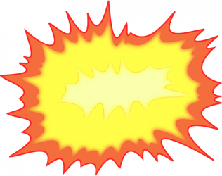
http://publicdomainvectors.org/en/free-clipart/Explosion-vector-illustration/7296.html
If there is a greater amount of matter in the original lump, the explosion will produce a denser cloud of debris. Its internal forces of gravitational attraction will be strong enough to slow and halt the initial outward motion of the explosion and draw the fragments back together, bringing about a collapse. It corresponds to the dynamics of cosmology I; there is a big bang and a big crunch.

If there is a lesser amount of matter in the original lump, the explosion will produce a more dilute debris cloud whose internal forces of attraction will not be sufficient to halt the initial outward motion of the blast. That outward motion will continue indefinitely. It corresponds to cosmology III; there is a big bang and no big crunch.

We could imagine an intermediate case in which the explosion is just energetic enough to fling the debris out of the reach of the gravitational forces; any weakening of the explosion would be too weak to prevent collapse. This corresponds to the intermediate case of cosmology II.
In all three cases, after the big bang, the mutual forces of gravitational attraction pull on the scattering debris. This decelerates their expansion and results in the downward pointing concavity of the curves of the scale factor R plotted above.
The Newtonian analogy is useful in so far as it gives us a nice picture for the dynamics. But it omits a lot. There is no account of the different spatial geometries and the big bang is the explosion of a nugget of matter into a pre-existing space. That is not what is portrayed by relativistic cosmologies.
The cosmic dynamics sketched above involve the simple case in which the cosmological constant Λ is zero. Our best astronomical evidence is that this constant is not zero; or at least the cosmos is behaving as if it is not zero. Let us now consider what happens when we have a non-zero cosmological constant.
| The main effect of a positive cosmological constant is to accelerate the expansion of the universe. In terms of the Newtonian analogy, a positive cosmological constant manifests as a repulsive force that leads galactic matter to move apart more rapidly than without the constant. It accelerates the expansion of the galaxies. | A negative constant manifests as an attractive force that further slows the expansion and makes collapse more likely. An anti-Sitter spacetime has a negative cosmological constant and collapses to a big crunch. |
We can see this acceleration in its purest form if we take the simplest case of a universe with a non-zero, positive cosmological constant, the de Sitter spacetime. We have already seen this spacetime earlier in the context of Einstein's earliest work in cosmology. It has no matter in it. We will below talk of small test bodies. We imagine them to have such tiny masses that they contribute negligibly. They are really just tell-tales to reveal the timelike geodesics of the spacetime.
To recall, the simplest way of creating a geometrically curved space is to start with a flat space and embed a curved surface in it. We arrived at a space with uniform positive curvature by embedding a sphere in a higher dimensional Euclidean space.
The de Sitter spacetime is the analog in relativity theory of this construction. That is, we start with a five-dimensional Minkowski spacetime, with one time dimension and four space dimensions. We embed a surface in it that is the analog of a sphere. That is, we embed in it a surface whose points are a constant spacetime interval from some central point. In the two dimensional case, the resulting figure would be a hyperbola, as we saw earlier. For the five dimensional case, the resulting figure is a four dimensional hyperboloid. It is drawn below, as best we can.

The difficulty with drawing the figure is that the full space is five dimensional, and the hyperboloid is a four dimensional figure. We can only give a drawing of it, if two of its four dimensions are suppressed. We show one dimension of time and one dimension of space. The de Sitter spacetime occupies the SURFACE of the hyperboloid, where I have used all caps to emphasize the point. The surface, if fully represented, would be four dimensional spacetime.
Space at any one moment in time is represented by one of the horizontal circles in the figure. Each circle is a one dimensional representation of a spherically curved three dimensional space of constant curvature. We read off the dynamics of the spacetime by tracing these circles as they evolve in time, from the bottom to the top of the figure. The three dimensional space collapses down to a smallest size and then expands outwards.
The vertical curves are the curves of test bodies of
negligible mass, that is, timelike geodesics.
They approach as the space contracts and then accelerate away from each
other. In this acceleration, we see the repulsive effect of the non-zero
cosmological constant at work. This motion is sometimes characterized as a
"bounce." The de Sitter spacetime is an expanding spacetime, where the
expansion does not originate in a singularity, but in a bounce after a
contraction phase.
We recover the three dimensional space of a spacetime by considering the spacetime at one moment of time. Geometrically this corresponds to slicing up the space with spatial hypersurfaces. Friedmann-Lemaitre-Robertson-Walker spacetimes generally admit a single, unique slicing. Here they differ from the Minkowski spacetime of special relativity. For the Minkowski spacetime, there are many equivalent ways of slicing up the spacetime. We saw that this is the geometric expression of the relativity of simultaneity. There is no relativity of simultaneity in Friedmann-Lemaitre-Robertson-Walker spacetimes, generally. The noteworthy exception is de Sitter spacetime. There are very many ways to slice up a de Sitter spacetime, so the relativity of simultaneity returns in this one special case.
There is something even more interesting: different ways of slicing up the de Sitter spacetime give us different geometries. We can slice up the spacetime so that we have spherical spaces of constant curvature, flat Euclidean spaces and hyperbolic spaces of constant negative curvature. Be careful: this is quite exceptional behavior! You will not find it in other Friedmann-Lemaitre-Robertson-Walker spacetimes.
| Here is the slicing implicit in the figure shown
earlier for a de Sitter spacetime. The hyperboloid is sliced by
horizontal planes that carve out spherical
spaces of constant curvature. They appear in the figure
just as circles. The slicing shown is done by a horizontal plane. That is just one of many that give a spherical space of constant curvature. The slicing plane can be tilted up or down and the same geometry for space will result. There is a limit to how far we can tilt the plane. Eventually, if we keep tilting it, we end up with the next case, shown below. |
 |
 |
If we tilt the hypersurface far enough,the geometry of the space
carved off changes. The moment is shown in the figure. The slicing
hypersurface is tilted far enough so the carved off space is no
longer closed. At the first moment that this happens, the space
carved off is a flat Euclidean space. To be a little more precise, the hyperboloid, if extended indefinitely, comes closer and closer to an ordinary cone. If the slicing hypersurface is parallel to one of the straight lines generating this cone, then the space carved off is Euclidean. This slicing is more limited than the first one above. If we try to introduce a cosmic time by slicing with many parallel hypersurfaces of this type, the slicing can cover only half the hyperboloid. Our new time coordinate will neglect the other half. |
| If we tilt still further, we come to the final case. The slicing
hypersurface intersects the hyperboloid in each of its lobes as
shown. The spaces carved off are hyperbolic
with constant negative curvature. As with the Euclidean space, if we use a set of these hypersurfaces to introduce a cosmic time, we can cover only half the hyperboloid. That the geometry of the de Sitter spacetime can be represented this simply is not easy to see from the literature. I found the simplest development, with figures analogous to these, in Roger Penrose, Fashion, Faith and Fantasy in the New Physics of the Universe. Princeton: Princeton University Press, 2016, pp. 222-23. |
 |
De Sitter spacetime represents a limiting case of special interest in cosmology. It is unrealistic in being matter free. However spacetimes with some matter, but whose dynamics of rapid expansion is driven by a cosmological constant, will resemble a de Sitter spacetime at least over some large patch.
The spacetime of the steady state cosmology of Bondi, Gold and Hoyle employed a de Sitter spacetime. Their slicing corresponded to the one that gives us Euclidean space, so that their spacetime exploited only half of the full de Sitter hyperboloid.
The three possibilities for cosmic dynamics considered above were generated with the assumption that the cosmological constant is zero. If we allow that it is not zero, how does the dynamics change? The main change is that a positive, non-zero cosmological constant accelerates the expansion of the galaxies, just as we saw in the special, matter free case of de Sitter spacetime. How much this affects the dynamics will depend upon the relative magnitudes of the constant and the density of ordinary matter (including radiation). The first accelerates the expansion; the second decelerates it. If the balance favors the cosmological constant, then we arrive at a universe that is accelerating overall. If we plot the growth of the scale factor R with time, we fill find new, accelerating time dependencies, as shown in the figure.

Otherwise, there are fewer changes. They are summarized here:
| What
does not change: There are still universes with the three geometries of ordinary, three-dimensional space of constant curvature: spherical, flat and hyperbolic. What determines the geometry of three-dimensional space is still the overall density of matter in relation to a critical density. In the comparison, the cosmological constant is treated as a form of matter. There are still universes with big bangs, some of which collapse to a big crunch and some of which do not. |
What
does change: The critical density no longer determines whether there is a big crunch. The most important factor is the cosmological constant. Almost any positive value leads to a universe without a big crunch. The density of ordinary matter has a secondary effect. There can be expanding universes with no big bang. They expand from a "bounce" after contraction in an earlier era. |
In all this, the range of possibilities is quite large,
according to the balance of cosmological constant and ordinary matter. A
now standard way to represent the range is through a diagram that appears
in many modern texts. It assumes that we are now in an expanding universe.
That fact enables a critical density to be computed from the Hubble
constant of the expansion.
• The density of ordinary matter now is represented as a fraction
of critical density, written in the figure as "Ωmatter,
now". Since the contribution of radiation to the ordinary
matter density in our present epoch is negligible, it is assumed to be
zero in the construction of the diagram.
• Correspondingly, the size of the cosmological constant is scaled to the
critical density, according to the matter-like effects it produces, and is
written in the figure as "ΩΛ,
now".
What makes matter "ordinary" is that it consists of baryonic particles, like protons and neutrons, that exert attractive gravitational effects and decelerate the cosmic expansion. (Recall that here we neglect other sort of "ordinary" matter: radiation like electromagnetic radiation.) The cosmological constant, treated as a form of matter, is not "ordinary," since that form of matter has the odd property of exerting a negative pressure that accelerates the expansion.
| There are two axes in
the figure. The horizontal axis shows how much ordinary matter is in
the universe now. When Ωmatter, now equals one, the
ordinary matter density is equal to the critical density. The vertical axis shows the strength of the effects of the cosmological constant now in relation to the critical density. Any pair of values Ωmatter, now and ΩΛ, now picks out a point in the figure. The geometry of three-dimensional space of the corresponding universe and its dynamics can be read from the region in which each point is found. This figure is drawn from the analysis given in M. P. Hobson, G. P. Efstathiou and A. N. Lasenby, General Relativity: An Introduction for Physicists. Cambridge: Cambridge University Press, 2006. Section 15.4. I found this treatment to be the most thorough. In particular, the formulae fixing some of the curves in the figure are quite complicated. This text goes to the trouble of deriving them and giving their explicit forms. For reference, for those who care, I have included the formulae in a version of the figure here. |
 |
 |
Let us start to read the diagram. The "closed/open" line refers to the geometry of ordinary, three-dimensional space. It divides those universes that have closed, spherical geometry from those with an open, flat or hyperbolic geometry. The line itself is just the set of all universes for which the sum of the ordinary and cosmological constant matter densities is exactly the critical density. We have already seen in the case of a zero cosmological constant that increasing the ordinary matter density makes it more likely that the geometry will be closed. That is replicated in the figure. Moving towards the right increases the ordinary matter density and, at the same time, moves us out of the red "open" region into the blue "closed" region. We see a similar effect with increasing cosmological constant, that is, as we move up in the figure. Larger cosmological constants move us up into the blue "closed" regions of a closed geometry of ordinary, three-dimensional space. |
| The line dividing the figure into green and
purple zones indicates when we will have recollapse
(a big crunch) or no collapse (no big crunch). The strongest, influencing factor is the value of the cosmological constant. Roughly speaking, almost any positive value for the cosmological constants puts us in the green, no recollapse region. That is not unexpected. The cosmological constant accelerates expansion, which drives the universe away from a big crunch. The purple region is, roughly, the region of negative cosmological constant. When it has a negative value, the cosmological constant acts attractively and decelerates the cosmic expansion. That is, it acts like ordinary matter, which also decelerates the expansion. The combined effect is to make recollapse and a big crunch inevitable, independently of the density of ordinary matter. The diagram shows that, once we have a non-zero cosmological constant, the density of ordinary matter has virtually no effect on whether the universe has a big crunch or not. The dividing line between the no recollapse and collapse regions is almost horizontal, which means that changing ordinary matter density is unlikely to move us between the regions. There is however a slight effect, as the next figure shows. |
 |
The figure below is a 10x magnification in the vertical direction of the region around the line in the figure that separates the no recollapse and the recollapse regions. The left half of the line, from Ωmatter, now = 0 to Ωmatter, now = 1, is located at zero cosmological constant and is perfectly horizontal. That tells us that changes in the ordinary matter density in the region have no influence on recollapse. The line corresponds to the cosmologies II and III above. The spatially flat cosmology II occupies just one point at Ωmatter, now = 1 on the line. At this point, the ordinary matter density is exactly the critical density. Cosmologies III, with hyperbolic geometry, occupy the remaining part of this left half of the line, where the ordinary matter density is less than the critical density.
Once we move further to the right into zones where Ωmatter, now > 1 and the ordinary matter density is greater than the critical density, we enter the recollapse, big crunch zone. It is here that the cosmologies of I above will be found. A very slight positive cosmological constant, however, moves these cosmologies vertically up the diagram into a no recollapse zone, eliminating the big crunch. We see that the value of the cosmological constant need only be very small to have this effect, since the vertical scale of the figure has been greatly magnified.

This dominance of the cosmological constant derives from the way that it and various forms of matter density alter as the cosmic expansion proceeds. Radiation energy density dilutes with 1/R4. That is, when the scale R factor doubles, the radiation energy density is reduced by a factor of 1/24 = 1/16. The energy density of ordinary baryonic matter decreases with R as 1/R3. When the scale factor doubles, this energy density reduces only by the smaller factor of 1/23 = 1/8. Under repeated doublings of R, as the expansion of the universe proceeds, the density of ordinary baryonic matter must eventually exceed that of radiation.
The cosmological constant Λ is a constant. It does not alter at all as the expansion proceeds. Thus, in the competition between radiative matter, ordinary matter and a positive cosmological constant, the assured winner will be the positive cosmological constant. All that it needs to win is that the expansion proceeds long enough for the other forms to matter to be sufficiently diluted. The small region in the diagram of collapse with a positive cosmological constant is the exceptional region in which the expansion has not proceeded long enough for the cosmological constant to dominate.
| As we move up the figure and the value of the cosmological constant increases, its accelerating effect will eventually overcome the decelerating effect of ordinary matter. The line shown divides the regions into universes that decelerate (yellow) and those that accelerate (blue). The line inclines up to the right, since the density of ordinary matter is greater on the right. Therefore a greater cosmological constant is needed to overcome its decelerating effects. |  |
 |
With still larger values of the cosmological constant, its
repulsive powers become great enough to preclude even a big bang
origin of the expansion itself. Most of this region lies outside the
range of the diagram. We see just part of it in the upper left hand
corner. The universes in the blue "no big bang" region will behave qualitatively like the de Sitter spacetimes. That is, their expansion will derive not from a big bang, but from an earlier phase of contraction that avoided a big crunch in favor of a bounce into an expanding phase. De Sitter spacetimes, with various values of the cosmological constant, are on the very left edge of this region. That left edge corresponds to a region of zero ordinary matter density. |
For completeness, the proper spelling of Georges Lemaître is as given in this sentence. There is a circumflex over the i. However not all browsers display the i-circumflex and, instead, show an annoying "?." So, at the risk of offending Lemaître partisans, I have simply written his name with an ordinary i.
| These are the names attached in our history to the spacetimes of big bang cosmology. Four names is a lot. How is that four theorists discover the same thing at the same time? The explanation is simply that its time had come and the result was there for anyone with the theoretical competence to pick it up. | Which names are attached to these spacetimes varies across the literature. Sometimes the short "Robertson Walker spacetime" is used. Or perhaps it is the slightly longer "Friedmann Robertson Walker spacetime." Less commonly, "Friedmann Lemaitre spacetime" is used. |
It was an exciting time in the history of cosmology. In the years around 1930 when these theorists made their discoveries, two ideas came together. First was Einstein's general theory of relativity. Since Einstein's first universe model of 1917, it was clear that general relativity had opened new theoretical possibilities for theorizing on the universe as a whole. Second was the recognition of the expansion of the galaxies. Combine these two pieces and one naturally and automatically poses the problem: which spacetimes of general relativity conform with the observed expansion of the galaxies? The result, as we saw above, proved simple enough to derive, once one had mastered enough general relativity. So many found it.
That way of telling the story oversimplifies the situation. It was a time of energetic theorizing and striking creativity. Everyone had their own program, their favored avenues and approaches and their pet aversions. The computation of the "the FLRW spacetime" arose naturally as a small puzzle to be solved within this chaos of different ideas and approaches.
| One indicator of the distance between them and us is the treatment
of the initial "big bang" singularity. We take the singularity as an
automatic element in the FLRW spacetimes. It has long since ceased
to trouble us. This was not the attitude at that time. The idea that there was a singularity in spacetime in our quite recent past was bothersome and worse. Arthur Eddington, an influential figure of the time in astronomy and cosmology, was most colorful in his hesitations. He wrote: "Philosophically, the notion of a beginning of the present order of Nature is repugnant to me." Arthur Eddington "The End of the World (From the Standpoint of Mathematical Physics)" The Mathematical Gazette, 15 (1931), pp. 316-324 on p. 319. [possibly] reprinted as Nature, vol. 127 (1931) p. 447-453. |
 |
Georges Lemaitre was bolder. But not at first. In 1927, he speculated about a universe that melded Einstein's static universe of 1917 and the expanding universe of de Sitter. In Lemaitre's model, as we go back arbitrarily far into the past, the universe came arbitrarily close to an Einstein universe. It was for most of its past history an Einstein universe, near enough. However the Einstein universe is unstable. Being near enough to an Einstein universe cannot persist. The deviation from it, no matter how small, must grow. And grow it did in Lemaitre's model, until the universe had transitioned to a de Sitter spacetime, near enough.
 |
By 1931, Lemaitre's theorizing had become bolder.
In a letter to the journal Nature in 1931 (vol
127, p. 706), he directly addressed Eddington's suggestion
that a beginning is repugnant. In response, he
speculated--wildly--of a cosmic beginning consisting of just a
single quantum, in the sense of quantum theory. With this initial
state, he surmised: "the notions of space and time would altogether fail to have any meaning at all." He concluded with a repudiation of Eddington's sense of repugnance: "If this suggestion is correct, the beginning of the world happened a little before the beginning of space and time. I think that such a beginning of the world is far enough from the present order of Nature to be not at all repugnant." |
| The wrangling over the acceptability of an initial cosmic singularity persisted. It is even enshrined in the name. Fred Hoyle was one of the three founders of the steady state cosmology, in which the universe expanded constantly, but still with an infinite past. On March 28, 1947, he spoke on BBC Radio's "Third Program," where he described the initial singularity of the competing view as supposing the origin of the universe in a "big bang." Hoyle denied his intent was to disparage the notion, but his targets took the term as a badge of honor and popularized it. |  |
Which of all these cosmologies is ours? This is THE question that has been left to last. The answer to this question will tell us important things about our cosmology as a whole.
• Was there really a big bang?
• Will there be a big crunch in our distant future in which all matter, space and time are to be snuffed out in a final cataclysm?
• Will the universe continue to expand forever, diluting matter indefinitely into a cold, dark emptiness?
• Are we in a finite space? Or does space extend indefinitely in all directions?
• Which is the geometry of our space?
• Has Euclid's geometry survived the challenge of relativity on the cosmic scale?
The answers to these questions is given by determining the density of the various forms of matter in the universe in relation to the critical density. Before we proceed, it is worth taking a moment to grasp the magnitude of the critical density.
The value of the critical density is determined by the Hubble constant derived from the observed rate of expansion of the galaxies. The critical density is extremely small: it is roughly 10-29 grams per cubic centimeter of space. That is 0.00000000000000000000000000001 grams per cubic centimeter. That is very little indeed! It corresponds to roughly 5 hydrogen atoms only in a cubic meter of space. That sort of vacuum is extremely hard to achieve with laboratory equipment on earth.
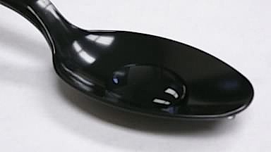 |
Here's another measure of how small it is. Take one
fifth of a teaspoon of water, which is roughly 20 drops.
(That amounts to one gram.) How widely spread must it be in order to
match the critical density? Guess! What if we take those 20 drops and spread them over the volume of the Astrodome? Not even close. Think bigger. What about 20 drops spread over the volume of earth? Better, but still too small. That density is still 100 times too big. Those 20 drops of water need to spread over one hundred earth volumes if their dilution is to match the critical density! That, at least, is what my sums show. The radius of the earth is about 6,366,000 meters. So its volume is 1.08 x 10²¹ m3, which comes to 1.08 x 1027 cubic centimeters. So one gram spread over this volume is still roughly 100 times too dense. |
Since this critical density is so small, you might think that our universe must have an average density more than critical. That would be jumping to conclusions. What counts is the density of matter averaged over all space. So we need to take the matter of the earth and spread it over the vast emptiness of space between stars and galaxies. And then the calculation gets more complicated because of the steady accumulation of evidence that a very substantial portion of the energy of our universe is "dark," so its existence is actually inferred indirectly from the gravitational effects it produces.
Decades of careful observational work have given us results that have stabilized over the last decade or two. These determinations are as follows. The values are approximate and are routinely adjusted slightly as new observations are made. However the values remain roughly as stated below.
| ΛCDM: The Lambda- Cold Dark Matter Model. | |
| 70% | "Dark Energy." 70% of
critical density. A positive, non-zero cosmological
constant manifests in an acceleration of the the galactic expansion.
A measurement of that acceleration enables us to work backwards to
the value of the cosmological constant. Measurements of the motion
of very distant type 1a supernovae in 1998 and later have shown that
the expansion is accelerating and at a considerable rate. The
acceleration fits with what a positive, non-zero cosmological
constant would bring about. While that is all we know, it has become routine, to treat this cosmological constant as an exotic form of matter. The identification persists in spite a failure to identify any independent manifestation of "dark energy" as a form of matter or to arrive at any cogent theory for its nature. If it is a form of matter, it would be the most common form of matter in the universe. This revival of the cosmological constant was not entirely welcome. After Einstein's renunciation of it in the early 1930s, it faded from cosmological theorizing as an aesthetically unappealing and even ad hoc addition. However observational results matter more than aesthetic hunches and they have prevailed. |
| +25% | "Dark Matter." 25% of
critical density. Galaxies are a system of stars bound
together by their mutual gravitational attraction. The stars of the
galaxy orbit in much the same way as planets orbit in our solar
system. It is possible to determine how much mass must be present to
enforce these orbits. When this is done by adding up the matter in
the luminous stars, we fall far short of the matter needed. The standard resolution is to assume that there is considerable further matter in the galaxies that is not luminous and thus invisible in our telescopes. To preserve the stability of the galaxies, the resulting "dark matter" would need to be so common as to be the second most common form of matter in the universe. Once again we face the awkwardness of having no independent means of detecting this form of matter, other than through its gravitational effects (such as in gravitational lensing) and no cogent theory for its nature. |
| +5% | Ordinary baryonic matter. 5% of critical density. The form of matter that is most directly measurable is the familiar protons, neutrons and the like that make up the ordinary matter of starts and planets. They are the next most common form of matter in the universe. |
| +0.005% |
Radiation. 0.005% of critical density. In the early, hot stages of cosmic expansion, the energy density of radiation dominated that of ordinary matter. However, as the expansion proceeded, the density of radiation diluted faster than ordinary matter. In the present epoch, it has diluted so far as to be barely detectible as the cosmic background microwave radiation. |
| 100% | When we sum these contributions, the result comes
out almost exactly to 100% of critical
density. That is, the total density of matter from all forms is the
critical density. It is tempting to say "exactly the critical
density." However no measurement is absolutely precise. All we can
say is that total density is so close to the critical density that
it is either critical or something very close to it. |
As indicated, these parameters taken together comprise the "Lambda-Cold Dark Matter" model of cosmology. It now so widely accepted that it is often described as the "standard model," mimicking the terminology used for the dominant theory in particle physics.
| We can return to our diagram to determine what
this outcome means for our big questions. In terms of the parameters
of the diagram, we have: For dark energy/cosmological constant, ΩΛ, now = 0.7 For matter, we have Ωmatter, now = 0.3 where the "matter" parameter is a sum of dark matter contribution of 25% and ordinary baryonic matter of 5%. That locates our universe in the red spot. We read from the figure that: Our universe expanded from a big bang and that its expansion is accelerating. There will be no big crunch. BUT Our combined dark energy and matter density locates us right on or very near to the curve that demarcates an open from closed geometry of space. We can guess which of these possibilities is ours, but--maddenly--the data leaves the question undecided. |
 |
Given the minuscule size of the critical density, it does seem unkind of nature to give us a density so close to critical, so that the big question of our cosmic spatial geometry remains unanswered. Nature had many orders of magnitude amongst which to choose, but still chose the troublesome value.
When coincidences like this happen, we seek explanations. One that has enjoyed considerable support is the notion of "inflationary cosmology." According to it, in a very early stage of the universe, prior to the radiation dominated phase, the universe underwent an extremely rapid phase of expansion. The dynamics looked like that of a de Sitter spacetime.
Proponents of inflationary cosmology argue that this inflationary phase explains many of the features of our universe. Inflation gives a mechanism for taking densities far from critical and driving them towards critical density. It also explains how it is possible for the matter distribution to be so uniform. In the very early, pre-inflationary phase, matter came to a uniform distribution at least locally. That local uniformity is then stretched out by the inflation to give us the uniform distribution we now see.
Whilst popular, inflationary cosmology remains debated. Since inflation must still start with some parameter values, critics object that it merely pushes the puzzle of the particular values back one stage, without really explaining them. More recently, as we saw earlier, the notable achievement of inflation has been to explain the profile of anisotropies in the cosmic background radiation. This too has recently been challenged by the claim that variants of inflationary theory could return any desired profile.
Copyright John D. Norton. March 2001; January 2007, February 16, 23, October 16, November 10, 2008, March 31, 2010; January 1, 2013; March 18, 2015. January 3, 2016. January 18, 28, October 16, 2017. April 17, 2020. February 5, March 22, 2022.