Problem
Air quality monitoring has seen increased public demand in recent years, especially in urban areas - as the links between air quality and public health come into sharp focus.
However, the spatial and temporal distribution of reliable air quality data is still lacking. Citizen Scientists deploying low-cost sensors have the potential to fill the spatial and temporal gaps left by sparsely distributed official air quality monitors.
However, the questionable reliability and accuracy of data collected by non-scientists using low-cost sensors has proved to be a hurdle in incorporating this data into environmental models.
Even though citizen science has been identified as a crucial avenue for collecting environmental data on the necessary temporal and spatial scales, there is still doubt about the reliability of the data that it produces.
In this project, we have attempted to leverage citizen science frameworks and low-cost sensors to inspect the accuracy of the sensor readings, and to find ways to calibrate them using existing nearby official and non-official air quality data from more expensive sensors.
Approach
Our initial plan was to calibrate our prototype devices by deploying them near an official Allegheny County Monitoring station and observing how closely the readings from the low-cost sensors matched up with official readings. If there was a simple calibration calculation we could apply at the source, we would then test the calibrated readings against the official readings and note the accuracy of the data from the low-cost sensors. We then planned to combine the insight from calibrating the sensors with additional data sources around the city (SmellPGH, temperature, humidtity) to produce the most accurate PM2.5 data from our devices. However, once the prototype devices were ready, we could not deploy them as planned and perform the calibration due to social-distancing orders owing to the spread of COVID-19.
Since the beginning of the COVID-19 pandemic and the need to follow social distancing guidelines, we were unable to complete all the tasks that we set out to complete. However, we modified our approach to make the best of our current situation and took the following steps:
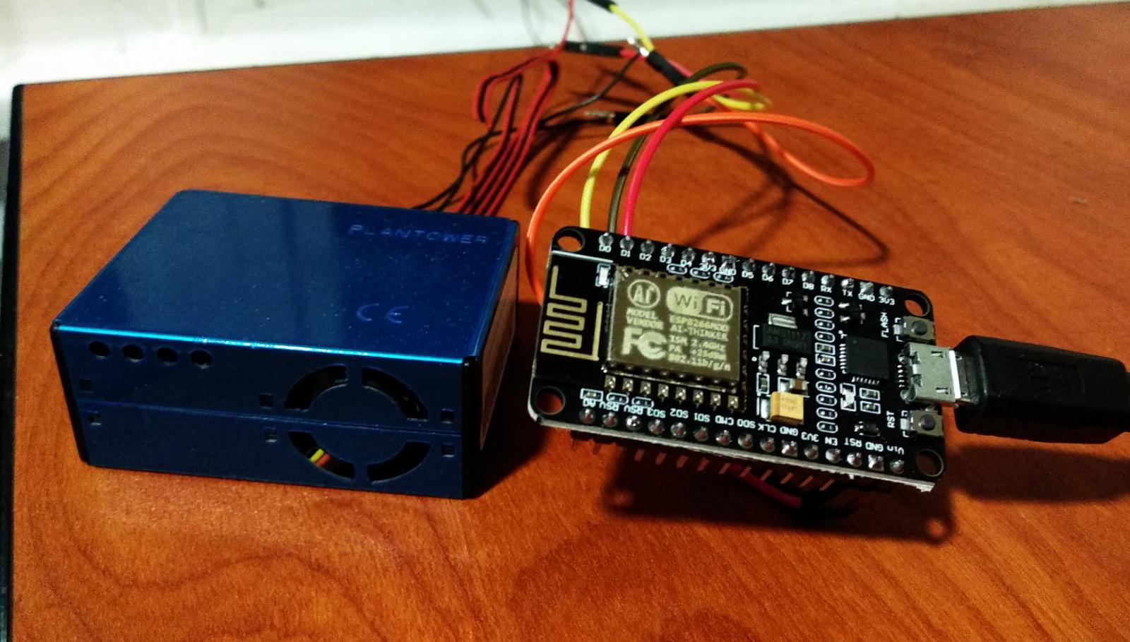
Build the prototype:
Using an Arduino ESP8266 device and a low-cost Plantower PMS5003 air quality sensor, we programmed the microprocessor to periodically collect PM0.3, PM0.5, PM1.0, PM2.5 and PM10 readings every 10 minutes. One prototype was deployed indoors in an apartment, and one was deployed outdoors - outside the window of the same apartment. These are named Maple and Pine respectively. They were connected to the home-wifi network of the apartment and the readings were sent to an online server that was set up to collect the readings.
Collect the readings:
The readings were collected in an online database hosted on Heroku. Readings were also collected using a Speck Indoor Air quality sensor.
Data pre-processing:
The official Allegheny County Monitors collect a variety of environmental data every hour. Each row of the dataset that is published contains 70 columns - with many of the columns very sparsely populated. Not wanting to discard a lot of freely available data, we chose certain well-populated columns for the duration of time that we were comparing the data, and then processed it to align with the closest time-stamped reading from our low-cost devices. However, since we were collecting data from our devices every 10 minutes, and Allegheny County publishes its data every 60 minutes, we had to settle for matching 6 readings from our devices to one reading from Allegheny County. It should also be noted that not only does the data have arbitrary gaps within columns, it is not consistent from monitor to monitor - while the Parkway East Monitor has 14 mostly-populated columns, the Avalon monitor only has 7, while other monitors have fewer or more columns of data. The bulk of the preprocessing was in eliminating null values, picking well-populated columns, changing formats of certain columns (time & date), and aligning them with data from our devices. Other datasets - like the Speck required conversion of Unix timestamps to our current timezone and elimination of 4 readings for every one of our readings, since it was programmed to collect data every 2 minutes. This data had to be manually downloaded and could not be accessed through an API. SmellPGH data was also downloaded and used - based on zipcodes that surrounded the zipcode of our low-cost sensors, we collected Smell reports and used the most recent smell-rating as an input field in our predictions. The following zipcodes were used - 15221, 15213, 15217, 15218, 15207, 15104, 15145, 15235, 15208, 15206, 15120, 15207, 15147, 15112.
Built a webpage to visualize the data:
A webpage was set up to easily access the data that was collected as well as visualize the data from other nearby sources. Data included Allegheny County Official Air Quality Monitors, PurpleAir Data from PurpleAir devices deployed by citizens and organizations around Pittsburgh, SmellPGH data (crowdsourced data with user-reported strong smells in the area) and data from our low-cost sensors (called PittAir on the website).
Results
We were able to successfully collect and save data from the prototypes as well as data from Allegheny County and a nearby PurpleAir monitor in our online database. 50 most recent readings can be accessed at: http://cs3551-airquality.herokuapp.com/readings
We have also set up a server to automatically visualize real-time data, available at the following link:
http://cs3551-airquality.herokuapp.com/
Data was analyzed using Linear Regression and Random Forest Regression techniques. Models were trained to be able to predict ‘official’ data using low-cost sensor data. R^2 values and RMSE values are provided below:
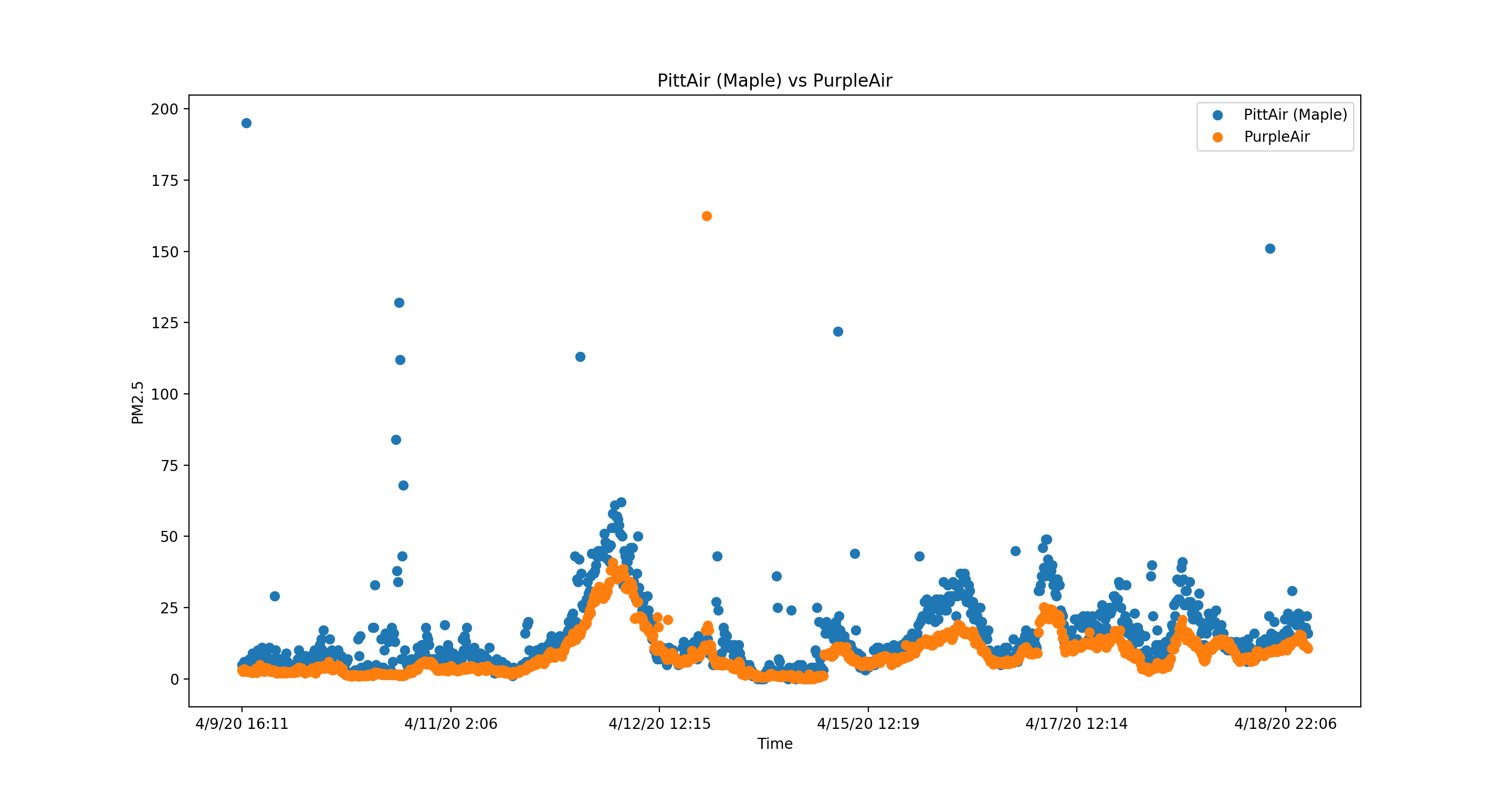
Using the data displayed on the graph above (with N=1022 datapoints), we trained a model using Random Forest Regression and we were able to obtain a model that had accuracy of 77%. The 1022 datapoints were split into 75% for training and 25% for testing. Accuracy is calculated using Coefficient of Determination with the following formula: (1 - u/v), where u is the residual sum of squares sum((y_true - y_pred)^2) and v is the total sum of squares sum((y_true - y_true.mean())^2).
Then using a new set of values with N=912 datapoints (that was not used in neither training nor testing), we obtained the following graphs. The graph on the left are the values without calibration (i.e. without using the model described above) and the graph on the right are the values after calibration. Without calibration we obtained a RMSE of 10.15 and after calibration we obtained a RMSE of 7.20.
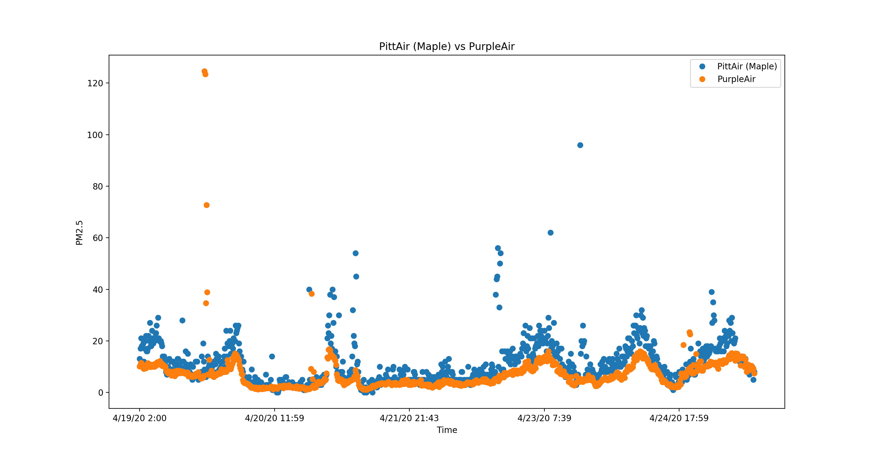
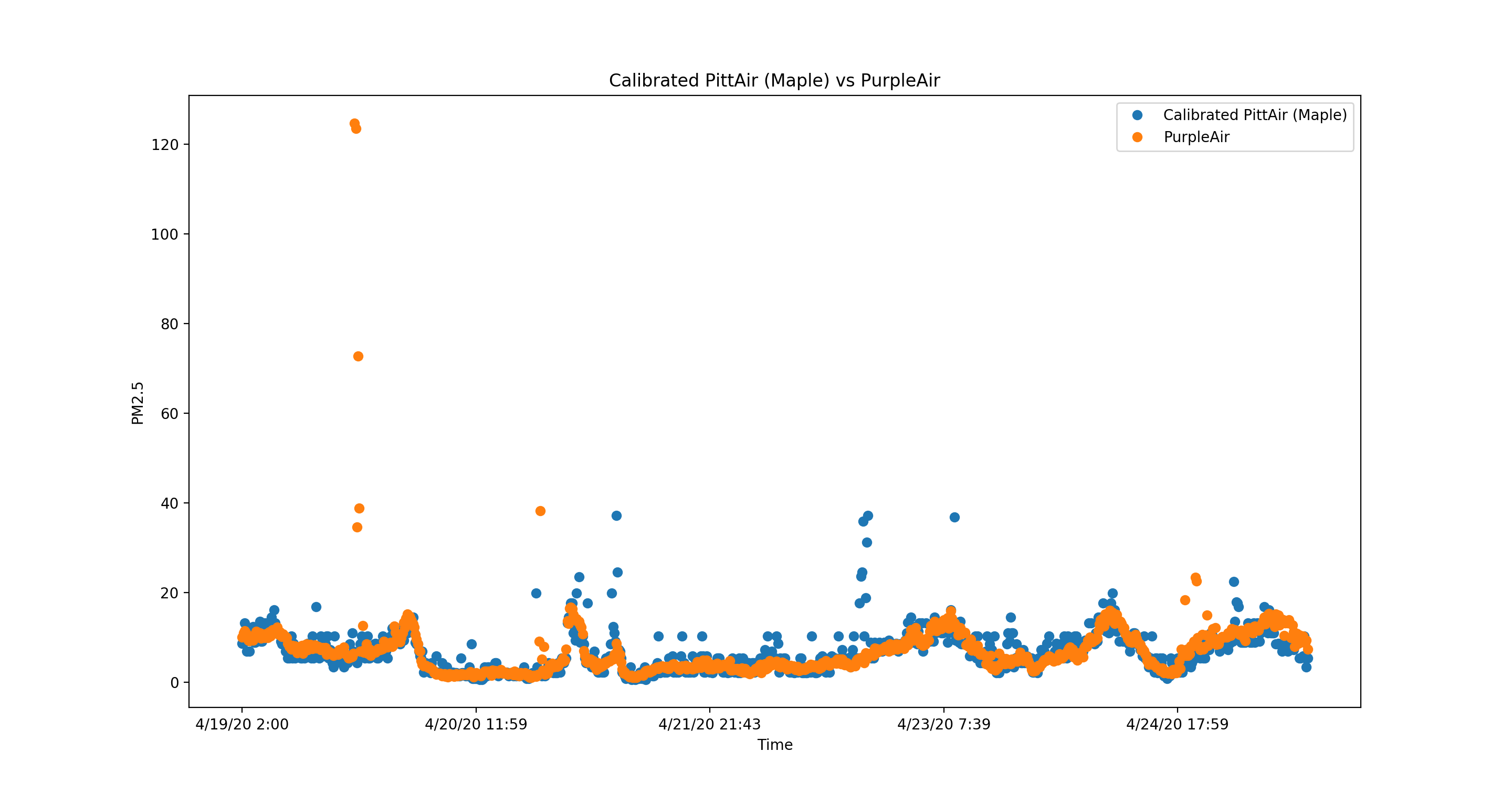
Visually, we can see that after calibrating the data using our model, the data aligns significantly better with PurpleAir data.
We also trained models using 4 different Regression techniques to analyze their RMSE values as a measure of their performance. The different models used were:
- Linear Regression
- Decision Tree
- Random Forest
- K-Nearest Neighbors
https://github.com/srnghn/ml_example_notebooks
The table below shows the size of the training dataset, the target variable, the maximum value of the target variable present in the dataset, and the RMSE values after 75% of the data was used to train the model and tested on the remaining 25% of the data. The analysis was done with SmellPGH data as an input and without, to observe the effect of this additional citizen-science based dataset.
Keywords:
- pred - predicting
- purpleair1, purpleair2 – PurpleAir devices’ data near the low-cost sensors (most likely indoors)
- w- with
- w/o – without
- smell – SmellPGH data
- speck – Speck Sensor data placed indoors in the same area as Maple
- acpe – Allegheny County Parkway East Monitor data
- acnb – Allegheny County North Braddock Monitor data
Note: The Linear Regression, Decision Tree, Random Forest, and KNN column values, in the table below,` refer to their RMSE.
| Training Size | Target Variable | Target Max | Linear Regression | Decision Tree | Random Forest | KNN | |
|---|---|---|---|---|---|---|---|
| pred-purpleair1-w-smell | 1451 | pu1_pm25_sorted | 162.47 | 4.6256 | 6.7012 | 4.2996 | 3.2449 |
| pred-purpleair1-w/o-smell | 1451 | pu1_pm25_sorted | 162.47 | 4.6342 | 6.872 | 6.7888 | 5.7572 |
| pred-purpleair2-w-smell | 1032 | pu2_pm25_sorted | 22.65 | 2.1273 | 2.3499 | 2.0339 | 2.1299 |
| pred-purpleair2-w/o-smell | 1032 | pu2_pm25_sorted | 22.65 | 2.1219 | 2.62488 | 2.1293 | 2.1119 |
| pred-speck-w-smell | 1451 | sp_part_con_sorted | 230.7 | 9.652 | 13.3078 | 10.1104 | 10.4322 |
| pred-speck-w/o-smell | 1451 | sp_part_con_sorted | 230.7 | 9.6502 | 10.6151 | 10.1183 | 10.1493 |
| pred-acpe-w-smell | 1744 | acpe_pm25t_sorted | 25 | 4.4963 | 6.1079 | 4.7647 | 4.7905 |
| pred-acpe-w/o-smell | 1744 | acpe_pm25t_sorted | 25 | 4.52 | 6.5098 | 5.1326 | 5.3463 |
| pred-acnb-w-smell | 1744 | acnb_pm10_sorted | 113 | 15.4251 | 20.1199 | 15.9284 | 11.612 |
| pred-acnb-w/o-smell | 1744 | acnb_pm10_sorted | 113 | 15.5431 | 22.1702 | 17.3178 | 11.4296 |
The target max column is helpful in contextualizing the RMSE values since it indicates the range of values that can be expected in prediction.
Here, we see that of all the models, K-Nearest Neighbor performs the best (has the lowest RMSE) in fitting the data, especially when SmellPGH data is used as one of the inputs during the training.
The RMSE of 3.2449 using KNN is 1.99% of the maximum observed value of the target variable, so we can say that the model performs reasonably well at predicting the values of the PurpleAir1 monitor.
Predicting PurpleAir2 PM2.5 data using low-cost indoor sensor (Maple):Here, we see that of all the models, Random Forest Regression performs the best (has the lowest RMSE) in fitting the data, when SmellPGH data is used as one of the inputs during the training.
The RMSE of 2.0339 using Random Forest Regression is 8.97% of the maximum observed value of the target variable, so this fit is fair, but could be improved.
Predicting Speck Sensor Particle Concentration using low-cost indoor sensor (Maple):Here, we see that of all the models, Linear Regression performs the best (has the lowest RMSE) in fitting the data, when SmellPGH data is excluded from the inputs during the training.
The RMSE of 9.6502 using Linear Regression is 4.18% of the maximum observed value of the target variable, so we can say that this is an acceptable fit.
Predicting Allegheny County (Parkway East) Monitor PM2.5 data using low-cost outdoor sensor (Pine):Here, we see that of all the models, Linear Regression performs the best (has the lowest RMSE) in fitting the data, when SmellPGH data is used as one of the inputs during the training.
The RMSE of 4.4963 using Linear Regression is 17.98% of the maximum observed value of the target variable and is not an acceptable result for environmental analysis. The model’s hyperparameters may be tuned or other models must be used, possibly along with other datasets in the training phase, to improve the prediction accuracy.
Predicting Allegheny County (North Braddock) Monitor PM1.0 data using low-cost outdoor sensor (Pine):Here, we see that of all the models, K-Nearest Neighbor performs the best (has the lowest RMSE) in fitting the data, when SmellPGH data is excluded from the inputs during the training.
The RMSE of 11.4296 using KNN is 10.11% of the maximum observed value of the target variable, so this fit is fair, but could be improved using different tuning parameters or additional data sources.
In most cases, we see a trend of lower RMSE values when the training dataset includes SmellPGH data – which is consistent with expectations of more data adding to greater accuracy. We can say that given the spatial variations in the data collected, the predictions of the Allegheny County Monitor data are less than ideal, but this could partially be attributed to differences in Particulate Matter Concentrations between the different areas. For the indoor monitors that are spatially much closer, we find predictions with reasonable RMSE values that can be improved upon to give a much better fit.
Future Work
There are many potential avenues to improve upon this work.
- Other Machine Learning-based Regression techniques could be used to better fit the data and predict more accurate values.
- More data sources (like local temperature, humidity) that affect the air quality measurements could be included in the training dataset.
- Hyper-parameters in the regression models used can be tuned to provide a better fit of the existing data.
- More data can be collected from all the sources. While each model was trained with at least 1000 data points, we believe the accuracy can be greatly improved with additional data. Especially since Allegheny County Monitors only collect and post data on an hourly basis.
- Spatial variations in data can be accounted for by placing a network of low-cost sensors between two ‘official’ sensors. This could give us valuable information about which data is ‘inaccurate’ and which data is simply different.