| front |1 |2 |3 |4 |5 |6 |7 |8 |9 |10 |11 |12 |13 |14 |15 |16 |17 |18 |19 |20 |21 |22 |23 |24 |25 |26 |27 |28 |29 |30 |31 |32 |33 |34 |35 |36 |37 |38 |39 |40 |41 |review |
 |
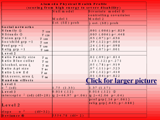
TABLE 3 (Cont):
Random intercept model, hierarchical linear regression of Alameda Physical Health Profile
on personal habits, social connections, and relative inequality, Moscow, 1991 Appendix II: The multilevel equation for the Alameda Physical Health Profile is similar to an ordinary least squares regression, except for including both individual level variables and urban area level variables in the same equation, and a complex error term: Yij =[ g 00 + g p0Xpij + g 0qZqj + g pqZqjXpij ]+[ u1jXpij + u0j + eij ], where Yij is the level of physical health for individual i in urban area j; p is the number of explanatory variables X for individual i; q is the number of explanatory variables Z at urban area j; ij=individual observation i in urban area j; Zqj=cross-level or micro-macro interaction, as the value of Y-X slope at the individual level with Z at the urban level. The fixed component of the regression, which is invariate between urban areas, is contained in the first set of parentheses. The complex error term within the second set of parentheses denotes the random component of the regression or the residual variation between urban areas, after the individual level variables are controlled. If there is no contextual effect and the residual variation is explained entirely by the fixed component, the hierarchical linear regression will produce the same results as an ordinary least squares solution. |