The explicit methods that we discussed last time are well suited to handling a large class of ODE's. These methods perform poorly, however, for a class of ``stiff'' problems that occur all too frequently in applications. We will examine implicit methods that are suitable for such problems. We will find that the implementation of an implicit method has a complication we didn't see with the explicit method: a (possibly nonlinear) equation needs to be solved.
The term ``stiff'' as applied to ODE's does not have a
precise definition. Loosely, it means that there is a very wide range
between the most rapid and least rapid (with ![]() ) changes in
solution components. A reasonably good rule of thumb is that if
Runge-Kutta or Adams-Bashforth or other similar methods require much
smaller steps than you would expect, based on your expectations for
the solution accuracy, then the system is probably stiff. The term
itself arose in the context of solution for the motion of a stiff
spring when it is being driven at a modest frequency of oscillation.
The natural modes of the spring have relatively high frequencies, and
the ODE solver must be accurate enough to resolve these high
frequencies, despite the low driving frequency.
) changes in
solution components. A reasonably good rule of thumb is that if
Runge-Kutta or Adams-Bashforth or other similar methods require much
smaller steps than you would expect, based on your expectations for
the solution accuracy, then the system is probably stiff. The term
itself arose in the context of solution for the motion of a stiff
spring when it is being driven at a modest frequency of oscillation.
The natural modes of the spring have relatively high frequencies, and
the ODE solver must be accurate enough to resolve these high
frequencies, despite the low driving frequency.
I've warned you that there are problems that defeat the explicit Runge-Kutta and Adams-Bashforth methods. In fact, for such problems, the higher order methods perform even more poorly than the low order methods. These problems are called ``stiff'' ODE's. We will only look at some very simple examples.
Consider the differential system
 |
|||
 |

The ODE becomes stiff when
We will be using this stiff differential equation in the exercises below, and in the next section you will see a graphical display of stiffness for this equation.
One way of looking at a differential equation is to plot its
``direction field.'' At any point ![]() , we can plot a
little arrow
, we can plot a
little arrow ![]() equal to the slope of the solution at
equal to the slope of the solution at ![]() .
This is effectively the direction that the differential equation is
``telling us to go,'' sort of the ``wind direction.''
How can you find
.
This is effectively the direction that the differential equation is
``telling us to go,'' sort of the ``wind direction.''
How can you find ![]() ? If the differential equation is
? If the differential equation is
![]() ,
and
,
and ![]() represents
represents ![]() ,
then
,
then
![]() , or
, or
![]() for a sensibly-chosen value
for a sensibly-chosen value ![]() . Matlab has some
built-in functions to generate this kind of plot.
. Matlab has some
built-in functions to generate this kind of plot.
function fValue = stiff4_ode ( x, y )
% fValue = stiff4_ode ( x, y )
% computes the right side of the ODE
%   dy/dx=f_ode(x,y)=lambda*(-y+sin(x)) for lambda = 4
% x is independent variable
% y is dependent variable
% output, fValue is the value of f_ode(x,y).

LAMBDA=4;
fValue = LAMBDA * ( -y + sin(x) );
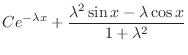
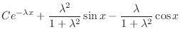
function y = stiff4_solution ( x )
% y = stiff4_solution ( x )
% computes the solution of the ODE
%   dy/dx=f_ode(x,y)=lambda*(-y+sin(x)) for lambda = 4
% and initial condition y=0 at x=0
% x is the independent variable
% y is the solution value

LAMBDA=4;
y = (LAMBDA^2/(1+LAMBDA^2))*sin(x) + ...
    (LAMBDA  /(1+LAMBDA^2))*(exp(-LAMBDA*x)-cos(x));
  h = 0.1;  % mesh size
  scale = 2.0; % make vectors longer
  [x,y] = meshgrid ( 0:h:2*pi, -1:h:1 );
  px = ones ( size ( x ) );
  py = stiff4_ode ( x, y );
  quiver ( x, y, px, py, scale )
  axis equal  %this command makes equal x and y scaling
  hold on
  x1=(0:h:2*pi);
  y1=stiff4_solution(x1);
  plot(x1,y1,'r')  % solution will come out red.
  hold off
Send me a copy of your plot (print -djpeg ex1.jpg, or File
x=linspace(0,2*pi,10);  % try 10, 20, 40, etc.
plot(x,stiff10000_solution(x))
Try it, but I think you will agree with me that it takes about 40 evenly-spaced points to make a reasonable curve. Do not send me copies of your plots.
The Backward Euler method is an important variation of Euler's method. Before
we say anything more about it, let's take a hard look at the
algorithm:
You might think there is no difference between this method and Euler's
method. But look carefully-this is not a ``recipe,'' the way
some formulas are. Since ![]() appears both on the left side
and the right side, it is an equation that must be solved for
appears both on the left side
and the right side, it is an equation that must be solved for
![]() , i.e., the equation defining
, i.e., the equation defining ![]() is implicit.
It turns out that implicit methods are much better suited to stiff
ODE's than explicit methods.
is implicit.
It turns out that implicit methods are much better suited to stiff
ODE's than explicit methods.
If we plan to use Backward Euler to solve our stiff ode equation,
we need to address the method of solution of the implicit equation
that arises. Before addressing this issue in general, we can treat
the special case:
function [x,y]=back_euler_lam(lambda,xRange,yInitial,numSteps)
% [x,y]=back_euler_lam(lambda,xRange,yInitial,numSteps)
% comments

% your name and the date.
that implements the above algorithm You may find it helpful to start out from a copy of your forward_euler.m file, but if you do, be sure to realize that this function has lambda as its first input parameter instead of the function name f_ode that forward_euler.m has. This is because back_euler_lam solves only the particular linear equation (3).
In the next exercise, we will compare backward Euler with
forward Euler for accuracy. Of course, backward Euler gives results when the
stepsize is large and Euler does not, but we are curious about the
case that there are enough steps to get answers.
Because it would require too many steps to run
this test with ![]() 1.e4, you will be using
1.e4, you will be using
![]() 55.
55.
abs( y(end) - stiff55_solution(x(end)) )Compute the ratios of the errors for each value of numSteps divided by the error for the succeeding value of numSteps. Use back_euler_lam to fill in the following table, over the interval [0,2*pi] and starting from yInit=0.
             lambda=55
numSteps back_euler_lam error   ratio
   40    ____________________  __________
   80    ____________________  __________
  160    ____________________  __________
  320    ____________________  __________
  640    ____________________  __________
 1280    ____________________  __________
 2560    ____________________
           lambda=55 Error comparison
numSteps  back_euler_lam        forward_euler
   40    ___________________   _________________
   80    ___________________   _________________
  160    ___________________   _________________
  320    ___________________   _________________
  640    ___________________   _________________
 1280    ___________________   _________________
 2560    ___________________   _________________
(In filling out this table, please include at least four
significant figures in your numbers. You can use
format long or format short e to get the desired precision.)
You should be convinced that implicit methods are worth while. How, then, can the resulting implicit equation (usually it is nonlinear) be solved? The Newton (or Newton-Raphson) method is a good choice. (We saw Newton's method last semester in Math 2070, Lab 4, you can also find discussions of Newton's method by Quarteroni, Sacco and Saleri in Chapter 7.1 or in a Wikipedia article http://en.wikipedia.org/wiki/Newton's_method.) Briefly, Newton's method is a way to solve equations by successive iterations. It requires a reasonably good starting point and it requires that the equation to be solved be differentiable. Newton's method can fail, however, and care must be taken so that you do not attempt to use the result of a failed iteration. When Newton's method does fail, it is mostly because the provided Jacobian matrix is not, in fact, the correct Jacobian for the provided function.
Suppose you want to solve the nonlinear (vector) equation

The superscript
There is an easy way to remember the formula for Newton's method. Write the finite difference formula for the derivative as
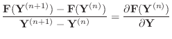
or, for vectors and matrices,
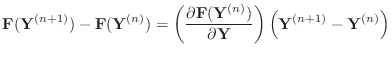
and then take
On each step, the backward Euler method requires a solution of the equation
so that we can take
I call your attention to a difficulty that has arisen. For the Euler,
Adams-Bashforth and Runge-Kutta methods, we only needed a function
that computed the right side of the differential equation. In order
to carry out the Newton iteration, however, we will also a
function that computes the partial derivative of the right side with
respect to ![]() . In 2070 we assumed that the derivative of
the function was returned as a second variable, and we will use
the same convention here.
. In 2070 we assumed that the derivative of
the function was returned as a second variable, and we will use
the same convention here.
To summarize, on each time step, start off the iteration by predicting the solution using an explict method. Forward Euler is appropriate in this case. Then use Newton's method to generate successive correction steps. In the following exercise, you will be implementing this method.
function [fValue, fPartial]=stiff10000_ode(x,y)
% [fValue, fPartial]=stiff10000_ode(x,y)
% comments

% your name and the date
and computes the partial derivative of stiff10000_ode with respect to y, fPartial. To do this, write the derivative of the formula for stiff10000_ode out by hand, then program it. attempt to use symbolic differentiation inside the function stiff1000_ode. Do not attempt to use symbolic differentiation inside the function stiff1000_ode.
function [x,y]=back_euler(f_ode,xRange,yInitial,numSteps)
% [x,y]=back_euler(f_ode,xRange,yInitial,numSteps) computes
% the solution to an ODE by the backward Euler method
%
% xRange is a two dimensional vector of beginning and
%   final values for x
% yInitial is a column vector for the initial value of y
% numSteps is the number of evenly-spaced steps to divide
%   up the interval xRange
% x is a row vector of selected values for the
%   independent variable
% y is a matrix. The k-th column of y is
%   the approximate solution at x(k)

% your name and the date

% force x to be a row vector
x(1,1) = xRange(1);
h = ( xRange(2) - xRange(1) ) / numSteps;
y(:,1) = yInitial;
for k = 1 : numSteps
  x(1,k+1) = x(1,k) + h;

  Y = (y(:,k)) + h * f_ode( x(1,k), y(:,k));
  [Y,isConverged]= newton4euler(f_ode,x(k+1),y(:,k),Y,h);

  if ~ isConverged
    error(['back_euler failed to converge at step ', ...
          num2str(k)])
  end

  y(:,k+1) = Y;
end
function [Y,isConverged]=newton4euler(f_ode,xkp1,yk,Y,h)
% [Y,isConverged]=newton4euler(f_ode,xkp1,yk,Y,h)
% special function to evaluate Newton's method for back_euler

% your name and the date

TOL = 1.e-6;
MAXITS = 500;

isConverged= (1==0);  % starts out FALSE
for n=1:MAXITS
  [fValue fPartial] = f_ode( xkp1, Y);
  F = yk + h * fValue - Y;
  J = h * fPartial - eye(numel(Y));
  increment=J\F;
  Y = Y - increment;
  if norm(increment,inf) < TOL*norm(Y,inf)
    isConverged= (1==1);  % turns TRUE here
    return
  end
end
% f_ode is the handle of a function whose signature is ???
% TOL = ??? (explain in words what TOL is used for)
% MAXITS = ??? (explain in words what MAXITS is used for)
% When F is a column vector and J a matrix,
  % the expression J\F means ???
% The Matlab function "eye" is used for ???
% The following for loop performs the spatial stepping (on x)
% The following statement computes the initial guess for Newton
f_ode=@stiff10000_ode, xkp1=2.0, yk=1.0,
h=0.1, and the initial guess Y=1,
write out by hand the (linear) equation that newton4euler solves.
To do this, start from (6), with
f_ode=@stiff10000_ode, xkp1=2.0, yk=1.0,
h=0.1, and the initial guess Y=1.
(If you discover that the Newton
iteration fails to converge, you probably have the derivative
in stiff10000_ode wrong.)
One simple nonlinear equation with quite complicated behavior is van der Pol's equation. This equation is written
where
As you know, van der Pol's equation can be written as a system of
first-order ODEs in the following way.
The matrix generalization of the partial derivative in Newton's method is the Jacobian matrix:
function [fValue, J]=vanderpol_ode(x,y)
% [fValue, J]=vanderpol_ode(x,y)
% more comments
% your name and the date

if numel(y) ~=2
  error('vanderpol_ode: y must be a vector of length 2!')
end

a=11;

fValue = ???

df1dy1 = 0;
df1dy2 = ???
df2dy1 = ???
df2dy2 = -a*(y(1)^2-1);

J=[df1dy1 df1dy2
   df2dy1 df2dy2];
be sure that fValue is a column and that the value
of the parameter
You have looked at the forward Euler and backward Euler methods. These methods are simple and involve only function or Jacobian values at the beginning and end of a step. They are both first order, though. It turns out that the trapezoid method also involves only values at the beginning and end of a step and is second order accurate, a substantial improvement. This method is also called ``Crank-Nicolson,'' especially when it is used in the context of partial differential equations. As you will see, this method is appropriate only for mildly stiff systems.
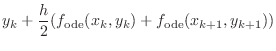
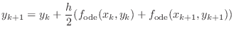
The trapezoid method can be derived from the trapezoid rule for
integration. It has a simple form:
In the exercise below, you will write a version of the trapezoid method using Newton's method to solve the per-timestep equation, just as with back_euler. As you will see in later exercises, the trapezoid method is not so appropriate when the equation gets very stiff, and Newton's method is overkill when the system is not stiff. The method can be successfully implemented using an approximate Jacobian or by computing the Jacobian only occasionally, resulting in greater computational efficiency. We are not going to pursue these alternatives in this lab, however.
function [ x, y ] = trapezoid ( f_ode, xRange, yInitial, numSteps )
% comments
[Y,isConverged]= newton4euler(f_ode,x(k+1),y(:,k),Y,h);with the new line
[Y,isConverged]=newton4trapezoid(f_ode,x(1,k),x(1,k+1),y(:,k),Y,h);
function [Y,isConverged]=newton4trapezoid(f_ode,xk,xkp1,yk,Y,h)
and replace
Modify newton4trapezoid.m to solve this function. Do not forget to modify the Jacobian J
f_ode=@stiff55_ode, xk=1.9, xkp1=2.0, yk=1.0,
h=0.1, and the initial guess for Y=1.
f_ode=@stiff55_ode, xk=1.9, xkp1=2.0, yk=1.0,
and h=0.1. Be sure your solution to this equation agrees with
the one from newton4trapezoid to at least 10 decimal places.
If not, find the mistake and fix it.
             stiff55
numSteps  trapezoid error         ratio
  10     ____________________  __________
  20     ____________________  __________
  40     ____________________  __________
  80     ____________________  __________
 160     ____________________  __________
 320     ____________________
In the following exercise, you are going to see that the difference in accuracy between the trapezoid method and the backward Euler method for solution of the vander Pol equation.
hold off
[x,y]=trapezoid(@vanderpol_ode,[0,10],[0;0],100);plot(x,y)
hold on
[x,y]=trapezoid(@vanderpol_ode,[0,10],[0;0],200);plot(x,y)
[x,y]=trapezoid(@vanderpol_ode,[0,10],[0;0],400);plot(x,y)
[x,y]=trapezoid(@vanderpol_ode,[0,10],[0;0],800);plot(x,y)
hold off
The trapezoid method is unconditionally stable, but this fact does not mean that it is good for very stiff systems. In the following exercise, you will apply the trapezoid method to a very stiff system so you will see that numerical errors arising from the initial rapid transient persist when using the trapezoid rule but not for backwards Euler.
Matlab has a number of built-in ODE solvers. These include:
| Matlab ODE solvers | |
| ode23 | non-stiff, low order |
| ode113 | non-stiff, variable order |
| ode15s | stiff, variable order, includes DAE |
| ode23s | stiff, low order |
| ode23t | trapezoid rule |
| ode23tb | stiff, low order |
| ode45 | non-stiff, medium order (Runge-Kutta) |
The ODE solvers we have written have four parameters, the function name, the solution interval, the initial value, and the number of steps. The Matlab solvers use a good adaptive stepping algorithm, so there is no need for the fourth parameter.
The Matlab ODE solvers require that functions such as vanderpol_ode.m return column vectors and there is no need for the Jacobian matrix. Thus, the same vanderpol_ode.m that you used for back_euler will work for the Matlab solvers. However, the format of the matrix output from the Matlab ODE solvers is the transpose of the one from our solvers! Thus, while y(:,k) is the (column vector) result achieved by back_euler on step k, the result from the Matlab ODE solvers will be y(k,:)!
ode45(@vanderpol_ode,[0,70],[0;0])Please include this plot with your summary.
figure(2)
ode45(@stiff10000,[0,8],1);
title('ode45')
figure(3)
ode15s(@stiff10000,[0,8],1);
title('ode15s')
You should be able to see that the step density (represented by the
little circles on the curves) is less for ode15s. This
density difference is most apparent in the smooth portions of
the curve where the solution derivative is small.
You do not need to send me these plots.
[x,y]=ode15s(@vanderpol_ode,[0,70],[0;0]);If you wish, you can plot the solution, compute its error, etc. For this solution, what is the value of
myoptions=odeset('RelTol',1.e-8);
[x,y]=ode15s(@vanderpol_ode,[0,70],[0;0],myoptions);
Use help odeset for more detail about options, and use the
command odeset alone to see the default options.
How many steps did it take this time? What is the value of Remark: The functionality of the Matlab ODE solvers is available in external libraries that can be used in Fortran, C, C++ or Java programs. One of the best is the Sundials package from Lawrence Livermore https://computation.llnl.gov/casc/sundials/main.html or odepack from Netlib http://www.netlib.org/odepack/.
You saw the Adams-Bashforth (explicit) methods in the previous lab. The
second-order Adams-Bashforth method (ab2) achieves higher order
without using intermediate points (as the Runge-Kutta methods do), but
instead uses points earlier in the evolution history, using the points
![]() and
and ![]() , for example, for ab2. Among implicit
methods, the ``backwards difference methods'' also achieve higher order
accuracy by using points earlier in the evolution history. It turns
out that backward difference methods are good choices for stiff problems.
, for example, for ab2. Among implicit
methods, the ``backwards difference methods'' also achieve higher order
accuracy by using points earlier in the evolution history. It turns
out that backward difference methods are good choices for stiff problems.
The backward difference method of second order can be written as
function [ x, y ] = bdm2 ( f_ode, xRange, yInitial, numSteps )
% [ x, y ] = bdm2 ( f_ode, xRange, yInitial, numSteps )
% ... more comments ...

% your name and the date
Although it would be best to start off the time stepping with a second-order method, for simplicity you should take one backward Euler step to start off the stepping. You should model the function on back_euler.m, and, with some ingenuity, you can use newton4euler without change. (If you cannot see how, just write a new Newton solver routine.)
Back to MATH2071 page.
![$\displaystyle J=\left[\begin{array}{cc} \frac{\partial f_1}{\partial y_1} & \fr...
...rtial f_2}{\partial y_1} & \frac{\partial f_2}{\partial y_2} \end{array}\right]$](img87.png)