In this lab we consider solution methods for ordinary differential equations (ODEs). We will be looking at two classes of methods that excel when the equations are smooth and derivatives are not too large. This lab will take two class sessions.
The lab begins with an introduction to Euler's (explicit) method for ODEs. Euler's method is the simplest approach to computing a numerical solution of an initial value problem. However, it has about the lowest possible accuracy. If we wish to compute very accurate solutions, or solutions that are accurate over a long interval, then Euler's method requires a large number of small steps. Since most of our problems seem to be computed ``instantly,'' you may not realize what a problem this can become when solving a ``real'' differential equation.
Applications of ODEs are divided between ones with space as the independent
variable and ones with time as the independent variable. We will
use ![]() as independent variable consistently. Sometimes it will
be interpreted as a space variable (
as independent variable consistently. Sometimes it will
be interpreted as a space variable (![]() -axis) and sometimes as
time.
-axis) and sometimes as
time.
A number of methods have been developed in the effort to get solutions that are more accurate, less expensive, or more resistant to instabilities in the problem data. Typically, these methods belong to ``families'' of increasing order of accuracy, with Euler's method (or some relative) often being the member of the lowest order.
In this lab, we will look at ``explicit'' methods, that is, methods
defined by an explicit formula for ![]() , the approximate solution
at the next time step, in terms of quantities derivable from previous
time step data. In a later lab, we will address ``implicit''
methods that require the solution of an equation in order to find
, the approximate solution
at the next time step, in terms of quantities derivable from previous
time step data. In a later lab, we will address ``implicit''
methods that require the solution of an equation in order to find
![]() . We will consider the Runge-Kutta and the Adams-Bashforth
families of methods. We will talk about some of the problems of
implementing the higher order versions of these methods. We will try
to compare the accuracy of different methods applied to the same
problem, and using the same number of steps.
. We will consider the Runge-Kutta and the Adams-Bashforth
families of methods. We will talk about some of the problems of
implementing the higher order versions of these methods. We will try
to compare the accuracy of different methods applied to the same
problem, and using the same number of steps.
Runge-Kutta methods are ``single-step'' methods while Adams-Bashforth
methods are ``multistep'' methods. Multistep methods require
information from several preceding steps in order to find ![]() and are a little more difficult to use. Nonetheless, both single and
multistep methods have been very successful and there are very
reliable Matlab routines (and libraries for other languages) available
to solve ODEs using both types of methods.
and are a little more difficult to use. Nonetheless, both single and
multistep methods have been very successful and there are very
reliable Matlab routines (and libraries for other languages) available
to solve ODEs using both types of methods.
Matlab vectors can be either row vectors or column vectors. Unlike
ordinary vectors in theoretical work, row and column vectors behave
almost as if they belong to different vector spaces. They cannot,
for example be added together and a matrix can only be multiplied
on the right by a column vector or on the left by a row vector.
The reason for the distinction is that vectors are really special
cases of matrices with a ``1'' for the other dimension. A row
vector of length ![]() is really a
is really a ![]() matrix and a column
vector of length
matrix and a column
vector of length ![]() is really a
is really a ![]() matrix.
matrix.
You should recall that row vectors are separated by commas when using square brackets to construct them and column vectors are separated by semicolons. It is sometimes convenient to write a column vector as a column. In the following expressions
rv = [ 0, 1, 2, 3];
cv = [ 0; 1; 2; 3; 4];
cv1 = [0
       1
       2
       3
       4];
The vector rv is a row vector and the vectors cv
and cv1 are column vectors.
If you do not tell Matlab otherwise, Matlab will generate a row vector when it generates a vector. The output from linspace is, for example, a row vector. Similarly, the following code
for j=1:10
  rv(j)=j^2;
end
results in the vector rv being a row vector. If you wish to generate a column vector using a loop, you can either first fill it in with zeros
cv=zeros(10,1);
for j=1:10
  cv(j)=j^2;
end
or use two-dimensional matrix notation
for j=1:10
  cv(j,1)=j^2;
end
A very simple ordinary differential equation (ODE) is the explicit
scalar first-order initial value problem:
An analytic solution of an ODE is a formula ![]() ,
that we can evaluate, differentiate, or analyze in any way we want.
Analytic solutions can only be determined for a small
class of ODE's. The term ``analytic'' used here is not quite the same
as an analytic function in complex analysis.
,
that we can evaluate, differentiate, or analyze in any way we want.
Analytic solutions can only be determined for a small
class of ODE's. The term ``analytic'' used here is not quite the same
as an analytic function in complex analysis.
A ``numerical solution'' of an ODE is simply a table of
abscissæ and approximate values
![]() that approximate the value of an analytic solution. This
table is usually accompanied by some rule for interpolating
solution values between the abscissæ.
With rare exceptions, a numerical solution is always wrong
because there is always some difference between the tabulated
values and the true solution. The
important question is, how wrong is it? One way to pose this question
is to determine how close the computed values
that approximate the value of an analytic solution. This
table is usually accompanied by some rule for interpolating
solution values between the abscissæ.
With rare exceptions, a numerical solution is always wrong
because there is always some difference between the tabulated
values and the true solution. The
important question is, how wrong is it? One way to pose this question
is to determine how close the computed values
![]() are to the analytic solution, which we might write as
are to the analytic solution, which we might write as
![]() .
.
The simplest method for producing a numerical solution of an ODE
is known as Euler's explicit method, or the forward
Euler method. Given a solution value
![]() ,
we estimate the solution at the next abscissa by:
,
we estimate the solution at the next abscissa by:
(The step size is denoted
Matlab note: In the following function, the name
of the function that evaluates ![]() is arbitrary. Recall that
if you do not know the actual name of a function, but it is
contained in a Matlab variable (I often use the variable name
``f_ode'')
then you can evaluate the function using the Matlab function
using the usual function syntax. Supposing you have a Matlab function
m-file named
my_ode.m and its signature line looks like the following.
is arbitrary. Recall that
if you do not know the actual name of a function, but it is
contained in a Matlab variable (I often use the variable name
``f_ode'')
then you can evaluate the function using the Matlab function
using the usual function syntax. Supposing you have a Matlab function
m-file named
my_ode.m and its signature line looks like the following.
function fValue=my_ode(x,y)Suppose you wish to call it from inside another function whose signature line looks like the following.
function [ x, y ] = ode_solver ( f_ode, xRange, yInitial, numSteps )When you call ode_solver using a command such as
[ x, y] = ode_solver(@my_ode,[0,1],0,10)then, inside ode_solver you can use syntax such as
fValue=f_ode(x,y)to call my_ode. This is the approach taken in this and future labs.
Matlab has an alternative, slightly more complicated, way to do the same thing. Inside ode_solver you can use the Matlab feval utility
fValue=feval(f_ode,x,y)to call my_ode.
Typically, Euler's method will be applied to systems of ODEs rather than a single ODE. This is because higher order ODEs can be written as systems of first order ODEs. The following Matlab function m-file implements Euler's method for a system of ODEs.
function [ x, y ] = forward_euler ( f_ode, xRange, yInitial, numSteps )
% [ x, y ] = forward_euler ( f_ode, xRange, yInitial, numSteps ) uses
% Euler's explicit method to solve a system of first-order ODEs
% dy/dx=f_ode(x,y).
% f = function handle for a function with signature
%    fValue = f_ode(x,y)
% where fValue is a column vector
% xRange = [x1,x2] where the solution is sought on x1<=x<=x2
% yInitial = column vector of initial values for y at x1
% numSteps = number of equally-sized steps to take from x1 to x2
% x = row vector of values of x
% y = matrix whose k-th column is the approximate solution at x(k).

x(1) = xRange(1);
h = ( xRange(2) - xRange(1) ) / numSteps;
y(:,1) = yInitial;
for k = 1 : numSteps
  x(1,k+1) = x(1,k) + h;
  y(:,k+1) = y(:,k) + h * f_ode( x(k), y(:,k) );
end
In the above code, the initial value (yInitial) is a column vector, and the function represented by f returns a column vector. The values are returned in the columns of the matrix y, one column for each value of x. The vector x is a row vector.
In the following exercise, you will use forward_euler.m to
find the solution of the initial value problem
function fValue = expm_ode ( x, y )
% fValue = expm_ode ( x, y ) is the right side function for
% the ODE dy/dx=-y+3*x
% x is the independent variable
% y is the dependent variable
% fValue represents dy/dx

fValue = -y-3*x;
yInit = 1.0;
[ x, y ] = forward_euler ( @expm_ode, [ 0.0, 2.0 ], yInit, numSteps );
for each of the values of numSteps in the table below. Use at least four significant figures when you record your numbers (you may need to use the command format short e), and you can use the first line as a check on the correctness of the code. In addition, compute the error as the difference between your approximate solution and the exact solution at x=2, y=-2*exp(-2)-3, and compute the ratios of the error for each value of nstep divided by the error for the succeeding value of nstep. As the number of steps increases, your errors should become smaller and the ratios should tend to a limit.
                  Euler's explicit method
numSteps Stepsize   Euler       Error       Ratio

   10     0.2     -3.21474836  5.5922e-02  _________
   20     0.1      __________  __________  _________
   40     0.05     __________  __________  _________
   80     0.025    __________  __________  _________
  160     0.0125   __________  __________  _________
  320     0.00625  __________  __________
Hint: Recall that Matlab has a special index, end,
that always refers to the last index. Thus, y(end)
is a short way to write y(numel(y)) when y is either
a row vector or a column vector.
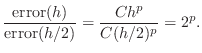 |
Based on the ratios in the table, estimate the order of
accuracy of the method, i.e., estimate the exponent
![]() in the error estimate
in the error estimate ![]() , where h is the step size.
, where h is the step size.
![]() is an integer in this case.
is an integer in this case.
The ``Euler halfstep'' or ``RK2'' method is a variation of Euler's
method. It is the second-simplest of a family of methods called ``Runge-Kutta''
methods. As part of each step of the method, an
auxiliary solution, one that we don't really care about, is computed
halfway, using Euler's method:
Although this method uses Euler's method, it ends up having a higher
order of convergence. Loosely speaking, the initial half-step provides
additional information: an estimate of the derivative in the middle of
the next step. This estimate is presumably a better estimate of the
overall derivative than the value at the left end point.
The per-step error is ![]() and, since there are
and, since there are
![]() steps to reach the end of the range,
steps to reach the end of the range, ![]() overall. Keep
in mind that we do not regard the auxiliary points as being part of
the solution. We throw them away, and make no claim about their
accuracy. It is only the whole-step points that we want.
overall. Keep
in mind that we do not regard the auxiliary points as being part of
the solution. We throw them away, and make no claim about their
accuracy. It is only the whole-step points that we want.
In the following exercise we compare the results of RK2 with Euler.
function [ x, y ] = rk2 ( f_ode, xRange, yInitial, numSteps )
% [ x, y ] = rk2 ( f_ode, xRange, yInitial, numSteps )
% comments including the signature, meanings of variables,
% math methods, your name and the date

x(1,1) = xRange(1);
h = ( xRange(2) - xRange(1) ) / numSteps;
y(:,1) = yInitial;
for k = 1 : numSteps
  xa = ??? ;
  ya = ??? ;
  x(1,k+1) = x(1,k) + h;
  y(:,k+1) = y(:,k) + h * f_ode( ??? );
end
                                  RK2
numSteps Stepsize   RK2          Error       Ratio

   10     0.2     -3.274896063 4.2255e-3   __________
   20     0.1      __________  __________  __________
   40     0.05     __________  __________  __________
   80     0.025    __________  __________  __________
  160     0.0125   __________  __________  __________
  320     0.00625  __________  __________
                       Euler
numSteps Stepsize      Error          RK2 Error

   10     0.2        __________      __________
   20     0.1        __________      __________
   40     0.05       __________      __________
   80     0.025      __________      __________
  160     0.0125     __________      __________
  320     0.00625    __________      __________
The idea in Euler's halfstep method is to ``sample the water''
between where we are and where we are going. This gives us a much
better idea of what ![]() is doing, and where our new
value of
is doing, and where our new
value of ![]() ought to be. Euler's method (``RK1'') and
Euler's halfstep method (``RK2'') are the junior members of a
family of ODE solving methods known as ``Runge-Kutta'' methods.
ought to be. Euler's method (``RK1'') and
Euler's halfstep method (``RK2'') are the junior members of a
family of ODE solving methods known as ``Runge-Kutta'' methods.
To develop a higher order Runge-Kutta method, we sample the
derivative function ![]() at even more ``auxiliary points''
between our last computed solution and the next one. These points are
not considered part of the solution curve; they are just a
computational aid. The formulas tend to get complicated, but let me
describe the next one, at least.
at even more ``auxiliary points''
between our last computed solution and the next one. These points are
not considered part of the solution curve; they are just a
computational aid. The formulas tend to get complicated, but let me
describe the next one, at least.
The third order Runge Kutta method ``RK3,'' given
![]() ,
, ![]() and a stepsize
and a stepsize ![]() , computes two intermediate points:
, computes two intermediate points:
The global accuracy of this method is ![]() , and
so we say it has ``order'' 3. Higher order Runge-Kutta
methods have been computed, with those of order 4 and 5 the most
popular.
, and
so we say it has ``order'' 3. Higher order Runge-Kutta
methods have been computed, with those of order 4 and 5 the most
popular.
function [ x, y ] = rk3 ( f_ode, xRange, yInitial, numSteps )
% comments including the signature, meanings of variables,
% math methods, your name and the date
that implements the above algorithm. You can use rk2.m as a model.
                                 RK3
numSteps Stepsize     RK3        Error        Ratio
   10     0.2      -3.27045877  2.1179e-04  __________
   20     0.1       __________  __________  __________
   40     0.05      __________  __________  __________
   80     0.025     __________  __________  __________
  160     0.0125    __________  __________  __________
  320     0.00625   __________  __________
numSteps Stepsize    RK2 Error       RK3 Error

   10     0.2        __________      __________
   20     0.1        __________      __________
   40     0.05       __________      __________
   80     0.025      __________      __________
  160     0.0125     __________      __________
  320     0.00625    __________      __________
fValue = expm_ode(1.0,[5;6])Please include the value of fValue in your summary file. If fValue is not a column vector of length 2, you have a mistake somewhere. Fix it before continuing. (Hint: First make sure your vector [5;6] has a semicolon in it and is a column vector.)
norm(ysystem(1,:)-y1)/norm(y1)  % should be roundoff or zero
norm(ysystem(2,:)-y2)/norm(y2)  % should be roundoff or zero
The equation describing the motion of a pendulum can be
described by the single dependent variable ![]() representing the angle the pendulum makes with the vertical.
The coefficients of the equation depend on the length of the
pendulum, the mass of the bob, and the gravitational constant.
Assuming a coefficient value of 3, the equation is
representing the angle the pendulum makes with the vertical.
The coefficients of the equation depend on the length of the
pendulum, the mass of the bob, and the gravitational constant.
Assuming a coefficient value of 3, the equation is
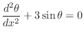
and one possible set of initial conditions is
 |
0 |
 |
|||
 |
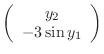
function fValue = pendulum_ode(x,y)
% fValue = pendulum_ode(x,y)
% comments including meanings of variables,
% math methods, your name and the date
Be sure to put comments after the signature line and wherever else they are needed. Be sure that you return a column vector.
     x   n          Euler                    RK3
   0.00  1     1.00      0.00         1.00        0.00
   6.25 ___  __________  __________   __________  __________
  12.50 ___  __________  __________   __________  __________
  18.75 ___  __________  __________   __________  __________
  25.00 ___  __________  __________   __________  __________
Hint: You may want to use the Matlab find
function. Use ``help find'' or the help menu for details.
You have seen a considerable amount of theory about stability of methods for ODEs, and you will see more in the future. Explicit methods generally are conditionally stable, and require that the step size be smaller than some critical value in order to converge. It is interesting to see what happens when this stability limit is approached and exceeded. In the following exercise you will drive Euler's method and Runge-Kutta third-order methods unstable using the expm_ode function from before. You should observe very similar behavior of the two methods. This behavior, in fact, is similar to that of most conditionally stable methods.
The message you should get from the previous exercise is that you can observe poor solution behavior when you are near the stability boundary for any method, no matter what the theoretical accuracy is. The ``poor behavior'' appears as a ``plus-minus'' oscillation that can shrink, grow, or remain of constant amplitude (unlikely, but possible). It can be tempting to accept solutions with small ``plus-minus'' oscillations that die out, but it is dangerous, especially in nonlinear problems, where the oscillations can cause the solution to move to a nearby curve with different initial conditions that has very different qualitative behavior from the desired solution.
Like Runge-Kutta methods, Adams-Bashforth methods want to estimate the behavior of the solution curve, but instead of evaluating the derivative function at new points close to the next solution value, they look at the derivative at old solution values and use interpolation ideas, along with the current solution and derivative, to estimate the new solution. This way they don't compute solutions at auxiliary points and then throw the auxiliary values away. The savings can result in increased efficiency.
Looked at in this way, the forward Euler method is the first order Adams-Bashforth method, using no old points at all, just the current solution and derivative. The second order method, which we'll call ``AB2,'' adds the derivative at the previous point into the interpolation mix. We might write the formula this way:
The AB2 method requires derivative values at two previous points,
but we only have one when starting out.
If we simply used an Euler step, we would pick up a relatively large
error on the first step, which would pollute all subsequent results. In
order to get a reasonable starting value, we should use the RK2
method, whose per-step error is order ![]() , the same
as the AB2 method.
, the same
as the AB2 method.
The following is a complete version of Matlab code for the Adams-Bashforth second-order method.
function [ x, y ] = ab2 ( f_ode, xRange, yInitial, numSteps )
% [ x, y ] = ab2 ( f_ode, xRange, yInitial, numSteps ) uses
% Adams-Bashforth second-order method to solve a system
% of first-order ODEs dy/dx=f_ode(x,y).
% f = name of an m-file with signature
%    fValue = f_ode(x,y)
% to compute the right side of the ODE as a column vector
%
% xRange = [x1,x2] where the solution is sought on x1<=x<=x2
% yInitial = column vector of initial values for y at x1
% numSteps = number of equally-sized steps to take from x1 to x2
% x = row vector of values of x
% y = matrix whose k-th row is the approximate solution at x(k).

x(1) = xRange(1);
h = ( xRange(2) - xRange(1) ) / numSteps;
y(:,1) = yInitial;

k = 1;
  fValue =  f_ode( x(k), y(:,k) );
  xhalf = x(k) + 0.5 * h;
  yhalf = y(:,k) + 0.5 * h * fValue;
  fValuehalf = f_ode( xhalf, yhalf );

  x(1,k+1) = x(1,k) + h;
  y(:,k+1) = y(:,k) + h * fValuehalf;

for k = 2 : numSteps
  fValueold=fValue;
  fValue = f_ode( x(k), y(:,k) );
  x(1,k+1) = x(1,k) + h;
  y(:,k+1) = y(:,k) + h * ( 3 * fValue - fValueold ) / 2;
end
   % The Adams-Bashforth algorithm starts here
   % The Runge-Kutta algorithm starts here
Be sure to include a copy of the commented code in your summary.
                                AB2
numSteps Stepsize  AB2(x=2)    Error(x=2)  Ratio

   10    0.2      -3.28013993  9.4694e-03  __________
   20    0.1       __________  __________  __________
   40    0.05      __________  __________  __________
   80    0.025     __________  __________  __________
  160    0.0125    __________  __________  __________
  320    0.00625   __________  __________
Adams-Bashforth methods try to squeeze information out of old solution points. For problems where the solution is smooth, these methods can be highly accurate and efficient. Think of efficiency in terms of how many times we evaluate the derivative function. To compute numSteps new solution points, we only have to compute roughly numSteps derivative values, no matter what the order of the method (remember that the method saves derivative values at old points). By contrast, a third order Runge-Kutta method would take roughly 3*numSteps derivative values. In comparison with the Runge Kutta method, however, the old solution points are significantly further away from the new solution point, so the data is less reliable and a little ``out of date.'' So Adams-Bashforth methods are often unable to handle a solution curve which changes its behavior over a short interval or has a discontinuity in its derivative. It's important to be aware of this tradeoff between efficiency and reliability!
You have seen above that some choices of step size ![]() result in
unstable solutions (blow up) and some don't. It is important to
be able to predict what choices of
result in
unstable solutions (blow up) and some don't. It is important to
be able to predict what choices of ![]() will result in unstable
solutions. One way to accomplish this task is to plot the region
of stability in the complex plane. An excellent source of further
information about stability regions can be found in Chapter Seven
of the book "Finite Difference Methods for Ordinary and Partial
Differential Equations" by Randall J. LeVeque at
will result in unstable
solutions. One way to accomplish this task is to plot the region
of stability in the complex plane. An excellent source of further
information about stability regions can be found in Chapter Seven
of the book "Finite Difference Methods for Ordinary and Partial
Differential Equations" by Randall J. LeVeque at
http://www.siam.org/books/ot98/sample/OT98Chapter7.pdf.
When applied to the test ODE
![]() , all of the common
ODE methods result in linear recurrance relations of the form
, all of the common
ODE methods result in linear recurrance relations of the form
It is a well-known fact that linear recursions of the form (7) have unique solutions in the form

where
The relationship between (7) and (8)
can be seen by assuming that, in the limit of large ![]() ,
,
![]() .
.
Clearly, the sequence ![]() is stable (bounded) if and only if
is stable (bounded) if and only if
![]() . Hence the ODE method associated with the
polynomial (8) is stable if and only if all the
roots satisfy
. Hence the ODE method associated with the
polynomial (8) is stable if and only if all the
roots satisfy
![]() .
.
The equation (8) can be solved (numerically if necessary)
for
![]() in terms of
in terms of ![]() .
Then, the so-called ``stability region,'' the set
.
Then, the so-called ``stability region,'' the set
![]() in the complex plane, can be plotted by plotting
the curve of those values of
in the complex plane, can be plotted by plotting
the curve of those values of ![]() with
with ![]() . This idea
can be turned into the following algorithmic steps.
. This idea
can be turned into the following algorithmic steps.
In the following exercise, you will implement this algorithm.
Replace the plot of the unit circle in your Matlab m-file with a plot
of the curve
![]() for 1000 points on the unit circle
for 1000 points on the unit circle
![]() . Include this plot in your summary file.
. Include this plot in your summary file.
Send me this second m-file and the plot with your summary.
Back to MATH2071 page.