MATH2071: LAB 1(b): Selected topics in Matlab
Introduction
This version of the first lab is intended only
for students who have already taken Math 2070.
There are two versions of the first lab. This version discusses
some special topics and is intended for students who took Math 2070.
If you have not already taken Math 2070,
That version of the first lab introduces
the Matlab environment and programming language, and presents the
general format of the work you need to hand in. Students who take
Lab 1(a) will be in no way disadvantaged in this course because
they ``missed'' Lab 1(b).
Grading policy for this semester has changed. Please refer to
for details.
This lab is concerned with several different topics. It covers material
that is supplemental for students in Math 2071, but new students
will not be shortchanged when they miss this material in favor of the
introductory material presented in Lab 1(a).
The first topic discussed in this lab is a simple approach in a
two-dimensional adaptive integration routine
using square mesh elements and
an elementary technique for determining which mesh elements need to be
refined in order to meet the error requirements.
The second topic is a demonstration of how roundoff error arises in
a matrix calculation.
The third topic is a brief introduction to ordinary differential equations.
This topic is also covered in Lab 1(a) and serves as an introduction to
the methods discussed in later labs.
Adaptive Quadrature
In this section you will construct a Matlab function to compute the
integral of a given mathematical function over a square region in the plane. One
way to do such a task would be to regard the square to be the
Cartesian product of two one-dimensional lines and integrate using
a one-dimensional adaptive quadrature routine such as adaptquad from
last semester. Instead, in this lab you will be looking at the
square as a region in the plane and you will be dividing it up into
many (square) subregions, computing the integral of the given function
over each subregion, and adding them up to get the integral over the
given square.
The basic outline of the method used in this lab is the following:
- Start with a list containing a single ``subregion'': the square region
of integration.
- Use a Gaußian integration rule to integrate the function
over each subregion in the list and estimate the resulting error of
integration. The integral over the whole region is the sum of the
integrals over the subregions, and similarly the estimated error is the
sum of the estimated errors over the subregions.
- If the total estimated error of the integral is small enough, the
process is complete. Otherwise, find the subregion with largest error,
replace it with four smaller subregions, and return to the previous step.
The way the notion of a ``list'' is implemented will introduce a
data structure (discussed in detail below) that is more versatile
than arrays or matrices.
Adaptive quadrature is build on quadrature and error estimation on a single
(square) element. The discussion starts there.
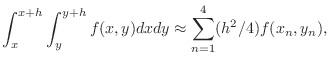
One simple way of deriving a two-dimensional integration formula
over a square is to use iterated integration. In this case, the
square has lower left coordinate  and side length
  , so
the square is
, so
the square is
![$ [x,x+h]\times[y,y+h]$](img3.png) .
Recall that a one-dimensional
Gauß integration rule can be written as
.
Recall that a one-dimensional
Gauß integration rule can be written as
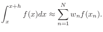 |
(1) |
Here,  is the index of the rule.
For the case
is the index of the rule.
For the case  , the points
  are
are
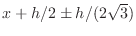 and the
weights are
and the
weights are
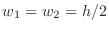 . The degree of precision is 3, and the
error is proportional to
. The degree of precision is 3, and the
error is proportional to
 . (If you look up the error
in a reference somewhere, you will notice that the error is usually
given as proportional to
. (If you look up the error
in a reference somewhere, you will notice that the error is usually
given as proportional to  , not
, not  . The extra power of
appearing in (1) comes from the fact that the
region of integration is
. The extra power of
appearing in (1) comes from the fact that the
region of integration is ![$ [x,x+h]$](img13.png) .) Applying (1) twice,
once in the
.) Applying (1) twice,
once in the  -direction and once in the
  -direction gives
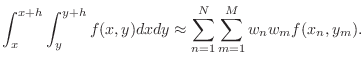 |
(2) |
For the case  , (2) becomes
 |
(3) |
where the four points
 .
These are four points based on the choices of ``
.
These are four points based on the choices of `` '' or ``
 '' signs.
Numbering the four choices is up to you.
The error is
'' signs.
Numbering the four choices is up to you.
The error is  over his
  square,
and (3) is exact for monomials
square,
and (3) is exact for monomials
 with
with  and
and  , and for sums of such monomials.
In the following exercise, you will implement this method in Matlab.
, and for sums of such monomials.
In the following exercise, you will implement this method in Matlab.
-
- Exercise 1:
- Write a Matlab function to compute the integral of a function
over a single square element using (3) with
. Name the
function m-file q_elt.m and have it begin
function q=q_elt(f,x,y,h)
% q=q_elt(f,x,y,h)
% INPUT
% f=???
% x=???
% y=???
% h=???
% OUTPUT
% q=???

% your name and the date
- Test qelt on the functions
 ,
,  ,
,  ,
,  , and
, and
 over the square
![$ [0,1]\times[0,1]$](img32.png) and show that the result is
exact, up to roundoff.
and show that the result is
exact, up to roundoff.
- Test qelt on the function
 to see that it is not
exact, thus showing the degree of precision is 3.
to see that it is not
exact, thus showing the degree of precision is 3.
In order to do any sort of adaptive quadrature, you need to be able to
estimate the error in one element. Remember, this is only an estimate
because without the true value of the quadrature, you cannot get the
true error.
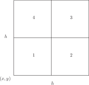
Suppose you have a square element with side of length
. If you
divide it into four sub-squares with sides of length  , then you
can compute the quadrature twice: once on the single square with side
of length
and once by adding up the four quadratures over the
four squares with sides of length
. Consider the following
figure.
, then you
can compute the quadrature twice: once on the single square with side
of length
and once by adding up the four quadratures over the
four squares with sides of length
. Consider the following
figure.
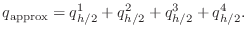
Denote the true integral over this square as  and its approximation
over the square with side of length
as
and its approximation
over the square with side of length
as  . Denote the four
approximate integrals over the four squares with sides of length
as
. Denote the four
approximate integrals over the four squares with sides of length
as  ,
,  ,
,  , and
, and  . Assuming that
the fourth derivatives of
. Assuming that
the fourth derivatives of  are roughly constant over the squares,
the following expressions can be written.
are roughly constant over the squares,
the following expressions can be written.
The second of these is assumed to be more accurate than the first,
so use it as the approximate integral,
 |
(5) |
The system of equations (4) can be solved for the error
in
 as
as
error in 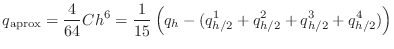 |
(6) |
In the following exercise you will write a Matlab function to
estimate both the integral and the error over a single element.
-
- Exercise 2:
- Write an m-file named qerr_elt.m
to estimate the both the integral
 approx
in (5)
and the error according to (6). Use
q_elt.m to evaluate the integrals.
qerr_elt.m should begin
approx
in (5)
and the error according to (6). Use
q_elt.m to evaluate the integrals.
qerr_elt.m should begin
function [q,errest]=qerr_elt(f,x,y,h)
% [q,errest]=qerr_elt(f,x,y,h)
% more comments

% your name and the date
- Use qerr_elt to estimate the integral and error
for the function
over the square
.
Since the exact integral is 1, and the method has degree of precision
equal to 3, both the error estimate and the true error should be
zero or roundoff.
- Use qerr_elt to estimate the integral and error
for the function
over the square
.
You should observe that the estimated error is within 5% of the
true error.
Up to now all the Matlab programs you have used involved fairly simple
ways of storing data, involving variables, vectors, and matrices. Another
valuable programming tool for storing data is the so-called ``structure.''
In many programming languages, such as Java, C and C++, it is called a
``struct,'' in Pascal it is called a ``record,'' and in Fortran, it is
called a ``defined type.'' In Matlab,
the term ``structure'' is used, although everyone will understand if you
call it a ``struct.''
You can find detailed information about structures in the Matlab
online documentation.
A structure consists of several named sub-fields, each containing a value,
and separated from the variable name with a dot. Rather than going into
full detail here, consider just the simple concept of a square region in
space, with sides parallel to the coordinate axes. Such a square can
be specified with three numerical quantities: the x and y coordinates
of the lower left corner point, and the length of a side. These three
quantities will be called x, y, and h for the purposes of this lab. Thus,
if a Matlab (structure) variable named elt were to refer to the
square
![$ [-1,1]\times[-1,1]$](img52.png) , it could be given as
, it could be given as
elt.x=-1;
elt.y=-1;
elt.h=2;
It is important to realize that the value of elt.x is unrelated
to the value of x that might appear elsewhere in a program.
For the purpose of this lab, two other quantities will be included in
this structure: the approximate integral of the function over this
element, called q, and the estimated error, called errest.
In the following exercises, you will be using a subscripted array (a vector) of
structures to implement the notion of a ``list of elements.'' Structures
can be indexed, and the resulting syntax for the
 th
entry of the
array of structures named elt would be elt(k). The
sub-fields of elt(k) are denoted
th
entry of the
array of structures named elt would be elt(k). The
sub-fields of elt(k) are denoted
elt(k).x
elt(k).y
elt(k).h
elt(k).q
elt(k).errest
-
- Exercise 3: In this exercise you will build up a function that estimates the
integral of a function and its error over a square by
choosing an arbitrary integer
 , and dividing the
square into
, and dividing the
square into  smaller squares, all the same size.
The point of this exercise is to introduce you to programming with structures.
Subsequent exercises will not use a uniform division of the square.
smaller squares, all the same size.
The point of this exercise is to introduce you to programming with structures.
Subsequent exercises will not use a uniform division of the square.
- Begin a function named q_total.m with the following code
template and correct the lines with ??? in them. This function
is incomplete: it ignores f and always computes the
area of the square, and estimates zero error.
function [q,errest]=q_total(f,x,y,H,n)
% [q,errest]=q_total(f,x,y,H,n)
% more comments
% n=number of intervals along one side

% your name and the date

h=( ??? )/n;
eltCount=0;
for k=1:n
  for j=1:n
    eltCount=eltCount+1;
    elt(eltCount).x= ???
    elt(eltCount).y= ???
    elt(eltCount).h= ???
    elt(eltCount).q= elt(eltCount).h^2; % to be corrected later
    elt(eltCount).errest=0;             % to be corrected later
  end
end
if numel(elt) ~= n^2
  error('q_total: something is wrong!')
end

q=0;
errest=0;
for k=1:numel(elt);
  q=q+elt(k).q;
  errest=errest+abs(elt(k).errest);
end
- Test the partially-written function q_total
by choosing any function f (since it is unused so far, it does
not matter) and using it to estimate the integral over the
square
using
 . Since it actually is computing
the area of the square, you should get 1.0. If you do not, you have
either computed the value of h incorrectly or you have
somehow generated the wrong number of elements. The length of
the vector elt should be precisely
.
. Since it actually is computing
the area of the square, you should get 1.0. If you do not, you have
either computed the value of h incorrectly or you have
somehow generated the wrong number of elements. The length of
the vector elt should be precisely
.
- As a second test, apply it to the square
using
 . Again, you should get the area of the square.
- Now that you have some confidence that the code has the correct
indexing,
use the function qerr_elt to estimate the
values of q and errest based on the elemental values of
x, y, and h and place them into
elt(elt_count).q and elt(elt_count).errest.
- Estimate the integral and error of the function
over the square
for the value
 .
If you do not get 1.0 with error estimate 0 or roundoff, you have computed
elt(elt_count).x or elt(elt_count).y or
elt(elt_count).h incorrectly or used qerr_elt incorrectly.
Note: numel(elt) is precisely 1 in this case.
.
If you do not get 1.0 with error estimate 0 or roundoff, you have computed
elt(elt_count).x or elt(elt_count).y or
elt(elt_count).h incorrectly or used qerr_elt incorrectly.
Note: numel(elt) is precisely 1 in this case.
- Estimate the integral and error of the function
over the square
for the value
.
If you do not get 4.0, you have computed
elt(elt_count).x or elt(elt_count).y. If your
estimated error is not zero or roundoff, you have likely
used qerr_elt incorrectly. Again,
numel(elt) is precisely 1 in this case.
- Estimate the integral and error of the function
over the square
for the value
 . If you do not
get 1, review your changes to q_total.m carefully.
. If you do not
get 1, review your changes to q_total.m carefully.
- Fill in the following table for the integral of the function
over the square
.
  n   integral    estimated error   true error
  2   ________     ____________     __________
  4   ________     ____________     __________
  8   ________     ____________     __________
 16   ________     ____________     __________
- Are your results consistent with the global order of
accuracy of
 ?
?
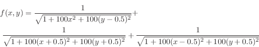
In order to further test the integration and error estimation,
a more complicated function is needed. One
function that is neither too easy nor too hard to integrate is
the following function.
This function has three peaks on the square
:
two at
 and one at
  . Its
integral over the square
is 1.755223755917299.
Matlab code to effect this function is:
. Its
integral over the square
is 1.755223755917299.
Matlab code to effect this function is:
function z=three_peaks(x,y)
% z=three_peaks(x,y)
% three peaks at (-.5,-.5), (+.5,-.5), (0,.5)
% the integral of this function over
%   [-1,1]X[-1,1] is 1.75522375591726

z=1./sqrt(1+ 100*(x+0.5).^2+ 100*(y+0.5).^2)+ ...
  1./sqrt(1+ 100*(x-0.5).^2+ 100*(y+0.5).^2)+ ...
  1./sqrt(1+ 100*(x    ).^2+ 100*(y-0.5).^2);
A perspective plot of the function is:
[scale=.5]lab01b_function.eps
-
- Exercise 4:
- Use cut-and-paste to copy the above code to a function m-file
named three_peaks.m.
- Integrate three_peaks over the square
using q_total
and fill in the following table. The true value of the integral
is 1.755223755917299. Warning: the larger values of
may
take some time--be patient.
  n   integral    estimated error   true error
 10   ________     ____________     __________
 20   ________     ____________     __________
 40   ________     ____________     __________
 80   ________     ____________     __________
160   ________     ____________     __________
- Are the true error values consistent with the convergence rate
of
?
- Notice that the estimated errors are much larger than the true
errors, especially for larger values of
. This is because the
elemental errors are sometimes positive and sometimes negative and
should cancel each other, but we take absolute values in the code
for q_total. Make a copy of q_total.m called
q_total_noabs.m and remove the absolute value from
the summation of the elemental error estimates. Using
q_total_noabs, compute the integral of three_peaks
over
using
 . You should observe that
the true and estimated errors agree within 0.1%. Nonetheless,
use of absolute value is adequate for smaller values of
and is
more conservative in all cases.
. You should observe that
the true and estimated errors agree within 0.1%. Nonetheless,
use of absolute value is adequate for smaller values of
and is
more conservative in all cases.
The objective of this discussion of quadrature is to present an
adaptive strategy for quadrature. You have seen all the pieces and
now it is time to put them together. In this strategy, a vector of
structures similar to the one used in q_total will be
used, but the way it is used is very different. The strategy
in q_total results in a large number of uniformly-sized
squares filling out the unit square. The adaptive stratgy below
will result in a smaller number of squares of differing sizes.
Small squares will be used only where they are needed to achieve
accuracy. The adaptive strategy used here is the following.
- Start with a vector named elt of structures similar to
the one used in
q_total above. This vector will have only one subscript:
elt(1).x
elt(1).y
elt(1).h
elt(1).q
elt(1).errest
and the values represent the given square region over which the
integral is to be taken, with elt(1).q and elt(1).errest
computed using qerr_elt.
- Add up all the elemental values of q and
absolute values of errest to get the total q
and errest. If errest is smaller than the tolerance,
stop and return the values of q and errest.
- If the total estimated error of the integral is too large,
find the value of k for which abs(elt(k).errest)
is largest and divide it into four subregions.
- Replace elt(k) with values from the upper right of
the four smaller square subelements. You can use code similar to
the following.
x=elt(k).x;
y=elt(k).y;
h=elt(k).h;

% new values for this element
elt(k).x=x+h/2;
elt(k).y=y+h/2;
elt(k).h=h/2;
[elt(k).q, elt(k).errest]=qerr_elt( ??? )
- Add three more elements to the vector of elements using code
similar to the following for each one.
K=numel(elt);
elt(K+1).x= ???
elt(K+1).y= ???
elt(K+1).h=h/2;
[elt(K+1).q, elt(K+1).errest]=qerr_elt( ??? )
- Go back to the second step above.
-
- Exercise 5:
- Write a Matlab function m-file named q_adaptive.m that
implements the preceeding algorithm. Your function could use the
following outline.
function [q,errest,elt]=q_adaptive(f,x,y,H,tolerance)
% [q,errest,elt]=q_adaptive(f,x,y,H,tolerance)
% more comments

% your name and the date
MAX_PASSES=500;

% initialize elt
elt(1).x=???
??? more code ???

for passes=1:MAX_PASSES
  % compute q by adding up elemental values
  % and compute errest by adding up absolute elemental values
  % use a loop for this because the "sum" function doesn't
  % work for structures.
  ??? more code ???

  % if error meets tolerance, return
  ??? more code ???

  % use a loop to find the element with largest abs(errest)
  ??? more code ???

  % replace that element with a quarter-sized element
  ??? more code ???

  % add three more quarter-sized elements
  ??? more code ???

end
error('q_adaptive convergence failure.');
- Test q_adaptive by computing the integral of the
function
over the square
to a tolerance
of 1.e-3. The result should be exactly correct because
the degree of precision is 3, and numel(elt) should be 1.
- Test q_adaptive by computing the integral of the
function
over the square
to a tolerance
of 1.e-3. The result should be exactly 4 because
the degree of precision is 3, and numel(elt) should be 1.
- Test q_adaptive by computing the integral of the
function
over the square
to a tolerance
of 1.e-3. You should see that numel(elt) is
precisely 4 because only a single refinement pass was required.
If you do not get the correct length, you can debug by
temporarily setting MAX_PASSES=2 in the code and look
at qelt. Is numel(qelt) equal to 4? If not, look at
the coordinates of each of the elements in elt. There should
be no duplicates or omissions. When you have corrected your error,
do not forget to reset MAX_PASSES=500
- Test q_adaptive by computing the integral of the
function
over the square
to a tolerance
of 2.e-4. You should see that numel(elt) is
precisely 7 because two refinement passes were required, with the
unit square broken into four subsquares and the upper right subsquare
itself broken into four.
In the following exercise you will see how the adaptive strategy
worked.
-
- Exercise 6:
- Download a plotting function
plotelt.m
that displays the elements. Elements colored green have small
estimated error, elements colored amber have mid-sized error
estimates and elements colored red have the largest error estimates.
Red elements are candidates for the next mesh refinement.
- Use q_adaptive to estimate the integral of the
function
over the square
to an
accuracy of 1.e-6. What are the integral, the estimated error,
and the true error? How many elements were used?
You should observe that the exact and estimated errors are close in size.
- Use plotelt to plot the final mesh used. Please include
a copy of this plot when you send me your work.
- Again estimate the integral of
over the square
, but to an accuracy of 9.e-7, smaller
than before. You should observe that the two large red blocks
near but not touching the origin have been refined.
Plot the resulting mesh, and include a copy with your summary.
- Again estimate the integral of
over the square
, but to an accuracy of 5.e-7.
You can see that
the red elements have been refined, green ones were not refined, and the
worst remaining elements are in different places.
-
- Exercise 7: Use q_adaptive to estimate the integral and error of
the function three_peaks over the square
to a tolerance of 1.e-5. Include the result, the estimated error,
the true error, and the number of mesh elements (numel(elt))
with your summary. Plot the resulting mesh and include
plot with your summary.
You should be able to see from the plot that elements near the peaks
themselves have been refined, but also elements in the areas between the
peaks.
Roundoff errors
Last term you saw some effects of roundoff errors. Later in this
term you will look at roundoff errors again. Right now, though,
is a good time to look at how some roundoff errors come about.
In the exercise below we will have occasion to use a special
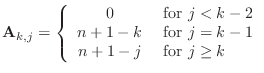
matrix called the Frank matrix.
Row  of the
  Frank matrix has the formula:
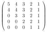
The Frank matrix for  looks like:
The determinant of the Frank matrix is 1, but is
difficult to compute numerically. This matrix has a special form called
Hessenberg form wherein all elements below the first subdiagonal
are zero. Matlab provides the Frank matrix in its ``gallery'' of
matrices, gallery('frank',n), but we will use an m-file
frank.m. The inverse of the
Frank matrix also consists of integer entries and an m-file for
it can be downloaded as
frank_inv.m.
You can find more information about the Frank matrix from the
Matrix Market,
and the references therein.
-
- Exercise 8: Let's look carefully at the
Frank matrix and its inverse. For convenience, define A to
be the Frank matrix of order 6, and Ainv its inverse, computed
using frank and frank_inv, respectively. Similarly,
let B and Binv be the Frank matrix of order 24 and its
inverse. Do not use the Matlab inv function for this exercise!
You know that both A*Ainv and B*Binv
should equal the identity matrices of order 6 and 24 respectively.
- What is the result of A*Ainv?
- What is the upper left
 square of C=B*Binv?
You should see that C is not a portion of the identity matrix.
What appears to be a mistake is actually the result of roundoff errors.
square of C=B*Binv?
You should see that C is not a portion of the identity matrix.
What appears to be a mistake is actually the result of roundoff errors.
- To see what is going on,
let's just look at the top left entry. Compute
  A(1,:)*Ainv(:,1)= __________
  B(1,:)*Binv(:,1)= __________
Both of these answers should equal 1. The first does and the second
does not.
- To see what goes right, compute the terms:
 A(1,6)*Ainv(6,1)= __________
 A(1,5)*Ainv(5,1)= __________
 A(1,4)*Ainv(4,1)= __________
 A(1,3)*Ainv(3,1)= __________
 A(1,2)*Ainv(2,1)= __________
 A(1,1)*Ainv(1,1)= __________
           sum   = __________
Note that the signs alternate, so that when you add them up,
each term tends to cancel part of the preceeding term.
- Now, to see what goes wrong, compute the terms:
 B(1,24)*Binv(24,1)= __________
 B(1,23)*Binv(23,1)= __________
 B(1,22)*Binv(22,1)= __________
 B(1,21)*Binv(21,1)= __________
 B(1,20)*Binv(20,1)= __________
 B(1,16)*Binv(16,1)= __________
 B(1,11)*Binv(11,1)= __________
 B(1,6) *Binv(6,1) = __________
 B(1,1) *Binv(1,1) = __________
You can see what happens to the sum. The first few
terms are huge compared with the correct value of 1. Matlab uses
64-bit floating point numbers, so you can only rely on the
first thirteen or fourteen significant digits in numbers like
B(1,24)*Binv(24,1).
Further, they are of opposing signs so that there is extensive
cancellation. There simply are not enough bits in the calculation to
get anything like the correct answer.
Remark: It would not have been productive to compute each of the
products B(1,k)*Binv(k,1) for each k, so I
had you do the five largest and then sampled the rest.
I chose to sample the terms with an
odd-sized interval between adjacent terms. Had I chosen
an even interval-say every other term-the alternating
sign pattern would have been obscured. When you are
sampling errors or residuals for any reason, never take
every other term!)
Ordinary differential equations
In this section you will see a brief introduction to
solving differential equations.
In general, a first-order ordinary differential equation can be written
in the form
 |
(7) |
where
 . Such an equation needs an initial condition
 . Perhaps the simplest method for numerically finding
a solution of (7) is to use the ``explicit Euler''
method wherein a discrete selection of points
. Perhaps the simplest method for numerically finding
a solution of (7) is to use the ``explicit Euler''
method wherein a discrete selection of points
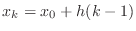 where
is some fixed step size and
where
is some fixed step size and
 . Writing the approximate
value of
. Writing the approximate
value of  as
as  , then Euler's explicit method can be derived
by approximating the derivative
, then Euler's explicit method can be derived
by approximating the derivative
 and writing
 |
(8) |
The differential equation
with initial condition  has an exact solution
 .
It also has an approximate numerical solution defined by Euler's
formula as
.
It also has an approximate numerical solution defined by Euler's
formula as
 |
(9) |
In some sense,
 We are going to look at how this expression evolves for
  .
.
-
- Exercise 9:
Copy the following text into a file named exer9.m
and then answer the questions about the code.
function error=exer9(nsteps)
% error=exer9(nsteps)
% compute the solution of the differential equation
% y'+y=sin(x)
% starting at y=0 at x=0 using Euler's method
% and ending at x=25
% nsteps=number of steps taken

% Your name and the date

FINAL_TIME=25.0;

stepsize=FINAL_TIME/nsteps;
clear x y exactSolution
y(1)=0;
x(1)=0;
exactSolution(1)=0;
for k=1:nsteps
  x(k+1)=x(k)+stepsize;
  y(k+1)=y(k)+stepsize*(-y(k)+sin(x(k)));
  exactSolution(k+1)=.5*(exp(-x(k+1))+sin(x(k+1))-cos(x(k+1)));
end
plot(x,y);  % default line color is blue
hold on
plot(x,exactSolution,'g'); % g for green line
legend('Euler solution','Exact solution')
hold off
error=norm(y-exactSolution)/norm(exactSolution);
- Add your name and the date to the comments at the beginning
of the file.
- Run exer9 with nsteps=160. You can see
that the approximate and exact solutions are quite close.
Please include this plot with your summary.
- Run exer9 with nsteps=10. You can see
that the approximate and exact solutions are not close and
are diverging from each other rapidly.
Please include this plot with your summary.
- Fill in the following table using exer9.
  nsteps      error       ratio
    10      _________    _______
    20      _________    _______
    40      _________    _______
    80      _________    _______
   160      _________    _______
The convergence rate should be
 for some
integer
for some
integer  . What is your estimate of
?
. What is your estimate of
?
Extra Credit (8 points)
You saw in Section 3 how roundoff errors can be generated
by adding numbers of opposite sign together. It is also possible to generate
roundoff by adding small numbers to large numbers, without sign changes. This
mechanism is not so dramatic as errors introduced by subtraction. In the
following exercise, you will see how roundoff errors can ge generated by
adding small numbers to large numbers and how roundoff can be mitigated by
grouping the smaller numbers together.
For this exercise, it will be convenient to use single
precision (32 bit) numbers rather than the usual double precision (64 bit)
numbers. This will show the effects of roundoff when using a much smaller
number of terms in the sum used below, resulting in much less time in
accumulating the sums.
Single precision numbers have only about eight significant digits, in
contrast to double precision numbers, which have about fifteen significant
digits.
The Matlab function single(x) returns a single
precision version of its argument x. Once single
precision numbers s1 and s2 have been generated,
they can be added (in single precision) in the usual manner
(s3=s1+s2), and the variable s3 will automatically be a single
precision variable. Even when another variable is a default (double)
precision number, adding it to or multiplying it by a single precision
number results in a single precision number.
Warning: For those who have programmed in other
languages, adding a single precision number to a double precision
number in Fortran or C results in a double precision value, not
single precision. Take care when mixing precisions in arithmetic
statements.
-
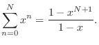
- Exercise 10: You probably have seen the formula for the sum of a geometric series.
 |
(10) |
Suppose that x=0.9999 and N=100000 ( ).
).
- Define a single precision variable x=single(0.9999).
- Compute the sum of the series 10 using the formula on
the right. Call this value S.
- Write a loop to accumulate the sum of the series (10)
by adding up the terms on the left. Call this value a.
- Write a loop to accumulate the sum of the series (10)
by adding up the terms on the left in reverse order
(for n=N:-1:0). Call this value b.
- Using format long, how many digits of a agree
with those of S? How many digits of b agree with those
of S? You should find that b is substantially closer
to S than a.
- Compute the relative errors abs((a-S)/S) and
abs((b-S)/S). You should find that the error in a is
more than 100 times the error in b.
- To see where the error comes from, compute the sum
 for
for
 terms. What is
?
What is the value of the next term in the series,
terms. What is
?
What is the value of the next term in the series,  ? When you
add
to
, there are only 8 digits of accuracy available,
so about four digits of the term
are lost in performing the sum!
Keeping this kind of loss up for thousands of terms is the source of
inaccuracy.
? When you
add
to
, there are only 8 digits of accuracy available,
so about four digits of the term
are lost in performing the sum!
Keeping this kind of loss up for thousands of terms is the source of
inaccuracy.
- Look at the reversed sum for b. In your own words, explain
why roundoff error is so much smaller in this case.
Back to MATH2071 page.
kimwong
2019-01-07