ABSTRACT
This chapter will provide an overview of Operations Research (O.R.)
from the perspective of an industrial engineer. The focus of the
chapter
is on the basic philosophy behind O.R. and the so-called "O.R.
approach"
to solving design and operational problems that industrial engineers
commonly
encounter. In its most basic form, O.R. may be viewed as a scientific
approach
to solving problems; it abstracts the essential elements of the problem
into a model, which is then analyzed to yield an optimal
solution
for implementation. The mathematical details and the specific
techniques
used to build and analyze these models can be quite sophisticated and
are
addressed elsewhere in this handbook; the emphasis of this chapter is
on
the approach. A brief review of the historical origins of O.R.
is
followed by a detailed description of its methodology. The chapter
concludes
with some examples of successful real-world applications of O.R.
INTRODUCTION
A HISTORICAL PERSPECTIVE
WHAT IS OPERATIONS RESEARCH
THE OPERATIONS RESEARCH APPROACH
Orientation
Problem Definition
Data Collection
Model Formulation
Model Solution
Validation and Analysis
Implementation and Monitoring
O.R. IN THE REAL WORLD
Harris Corporation
Texaco
Caterpillar
Delta Airlines
KeyCorp
SUMMARY
REFERENCES AND FURTHER READING
Although it is a distinct discipline in its own right, Operations Research (O.R.) has also become an integral part of the Industrial Engineering (I.E.) profession. This is hardly a matter of surprise when one considers that they both share many of the same objectives, techniques and application areas. O.R. as a formal subject is about fifty years old and its origins may be traced to the latter half of World War II. Most of the O.R. techniques that are commonly used today were developed over (approximately) the first twenty years following its inception. During the next thirty or so years the pace of development of fundamentally new O.R. methodologies has slowed somewhat. However, there has been a rapid expansion in (1) the breadth of problem areas to which O.R. has been applied, and (2) in the magnitudes of the problems that can be addressed using O.R. methodologies. Today, operations research is a mature, well-developed field with a sophisticated array of techniques that are used routinely to solve problems in a wide range of application areas.
This chapter will provide an overview of O.R. from the perspective of an Industrial Engineer. A brief review of its historical origins is first provided. This is followed by a detailed discussion of the basic philosophy behind O.R. and the so-called "O.R. approach." The chapter concludes with several examples of successful applications to typical problems that might be faced by an Industrial Engineer. Broadly speaking, an O.R. project comprises three steps: (1) building a model, (2) solving it, and (3) implementing the results. The emphasis of this chapter is on the first and third steps. The second step typically involves specific methodologies or techniques, which could be quite sophisticated and require significant mathematical development. Several important methods are overviewed elsewhere in this handbook. The reader who has an interest in learning more about these topics is referred to one of the many excellent texts on O.R. that are available today and that are listed under "Further Reading" at the end of this chapter, e.g., Hillier and Lieberman (1995), Taha (1997) or Winston (1994).
While there is no clear date that marks the birth of O.R., it is generally accepted that the field originated in England during World War II. The impetus for its origin was the development of radar defense systems for the Royal Air Force, and the first recorded use of the term Operations Research is attributed to a British Air Ministry official named A. P. Rowe who constituted teams to do "operational researches" on the communication system and the control room at a British radar station. The studies had to do with improving the operational efficiency of systems (an objective which is still one of the cornerstones of modern O.R.). This new approach of picking an "operational" system and conducting "research" on how to make it run more efficiently soon started to expand into other arenas of the war. Perhaps the most famous of the groups involved in this effort was the one led by a physicist named P. M. S. Blackett which included physiologists, mathematicians, astrophysicists, and even a surveyor. This multifunctional team focus of an operations research project group is one that has carried forward to this day. Blackett’s biggest contribution was in convincing the authorities of the need for a scientific approach to manage complex operations, and indeed he is regarded in many circles as the original operations research analyst.
O.R. made its way to the United States a few years after it originated in England. Its first presence in the U.S. was through the U.S. Navy’s Mine Warfare Operations Research Group; this eventually expanded into the Antisubmarine Warfare Operations Research Group that was led by Phillip Morse, which later became known simply as the Operations Research Group. Like Blackett in Britain, Morse is widely regarded as the "father" of O.R. in the United States, and many of the distinguished scientists and mathematicians that he led went on after the end of the war to become the pioneers of O.R. in the United States.
In the years immediately following the end of World War II, O.R. grew rapidly as many scientists realized that the principles that they had applied to solve problems for the military were equally applicable to many problems in the civilian sector. These ranged from short-term problems such as scheduling and inventory control to long-term problems such as strategic planning and resource allocation. George Dantzig, who in 1947 developed the simplex algorithm for Linear Programming (LP), provided the single most important impetus for this growth. To this day, LP remains one of the most widely used of all O.R. techniques and despite the relatively recent development of interior point methods as an alternative approach, the simplex algorithm (with numerous computational refinements) continues to be widely used. The second major impetus for the growth of O.R. was the rapid development of digital computers over the next three decades. The simplex method was implemented on a computer for the first time in 1950, and by 1960 such implementations could solve problems with about 1000 constraints. Today, implementations on powerful workstations can routinely solve problems with hundreds of thousands of variables and constraints. Moreover, the large volumes of data required for such problems can be stored and manipulated very efficiently.
Once the simplex method had been invented and used, the development of other methods followed at a rapid pace. The next twenty years witnessed the development of most of the O.R. techniques that are in use today including nonlinear, integer and dynamic programming, computer simulation, PERT/CPM, queuing theory, inventory models, game theory, and sequencing and scheduling algorithms. The scientists who developed these methods came from many fields, most notably mathematics, engineering and economics. It is interesting that the theoretical bases for many of these techniques had been known for years, e.g., the EOQ formula used with many inventory models was developed in 1915 by Harris, and many of the queuing formulae were developed by Erlang in 1917. However, the period from 1950 to 1970 was when these were formally unified into what is considered the standard toolkit for an operations research analyst and successfully applied to problems of industrial significance. The following section describes the approach taken by operations research in order to solve problems and explores how all of these methodologies fit into the O.R. framework.
A common misconception held by many is that O.R. is a collection of mathematical tools. While it is true that it uses a variety of mathematical techniques, operations research has a much broader scope. It is in fact a systematic approach to solving problems, which uses one or more analytical tools in the process of analysis. Perhaps the single biggest problem with O.R. is its name; to a layperson, the term "operations research" does not conjure up any sort of meaningful image! This is an unfortunate consequence of the fact that the name that A. P. Rowe is credited with first assigning to the field was somehow never altered to something that is more indicative of the things that O.R. actually does. Sometimes O.R. is referred to as Management Science (M.S.) in order to better reflect its role as a scientific approach to solving management problems, but it appears that this terminology is more popular with business professionals and people still quibble about the differences between O.R. and M.S. Compounding this issue is the fact that there is no clear consensus on a formal definition for O.R. For instance, C. W. Churchman who is considered one of the pioneers of O.R. defined it as the application of scientific methods, techniques and tools to problems involving the operations of a system so as to provide those in control of the system with optimum solutions to problems. This is indeed a rather comprehensive definition, but there are many others who tend to go over to the other extreme and define operations research to be that which operations researchers do (a definition that seems to be most often attributed to E. Naddor)! Regardless of the exact words used, it is probably safe to say that the moniker "operations research" is here to stay and it is therefore important to understand that in essence, O.R. may simply be viewed as a systematic and analytical approach to decision-making and problem-solving. The key here is that O.R. uses a methodology that is objective and clearly articulated, and is built around the philosophy that such an approach is superior to one that is based purely on subjectivity and the opinion of "experts," in that it will lead to better and more consistent decisions. However, O.R. does not preclude the use of human judgement or non-quantifiable reasoning; rather, the latter are viewed as being complementary to the analytical approach. One should thus view O.R. not as an absolute decision making process, but as an aid to making good decisions. O.R. plays an advisory role by presenting a manager or a decision-maker with a set of sound, scientifically derived alternatives. However, the final decision is always left to the human being who has knowledge that cannot be exactly quantified, and who can temper the results of the analysis to arrive at a sensible decision.
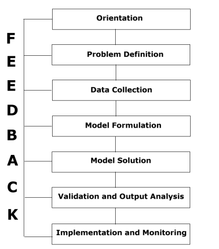
Given that O.R. represents an integrated framework to help make decisions, it is important to have a clear understanding of this framework so that it can be applied to a generic problem. To achieve this, the so-called O.R. approach is now detailed. This approach comprises the following seven sequential steps: (1) Orientation, (2) Problem Definition, (3) Data Collection, (4) Model Formulation, (5) Solution, (6) Model Validation and Output Analysis, and (7) Implementation and Monitoring. Tying each of these steps together is a mechanism for continuous feedback; Figure 1 shows this schematically.
While most of the academic emphasis has been on Steps 4, 5 and 6, the reader should bear in mind the fact that the other steps are equally important from a practical perspective. Indeed, insufficient attention to these steps has been the reason why O.R. has sometimes been mistakenly looked upon as impractical or ineffective in the real world.
Each of these steps is now discussed in further detail. To illustrate how the steps might be applied, consider a typical scenario where a manufacturing company is planning production for the upcoming month. The company makes use of numerous resources (such as labor, production machinery, raw materials, capital, data processing, storage space, and material handling equipment) to make a number of different products which compete for these resources. The products have differing profit margins and require different amounts of each resource. Many of the resources are limited in their availability. Additionally, there are other complicating factors such as uncertainty in the demand for the products, random machine breakdowns, and union agreements that restrict how the labor force can be used. Given this complex operating environment, the overall objective is to plan next month's production so that the company can realize the maximum profit possible while simultaneously ending up in a good position for the following month(s).
As an illustration of how one might conduct an operations research study to address this situation, consider a highly simplified instance of a production planning problem where there are two main product lines (widgets and gizmos, say) and three major limiting resources (A, B and C, say) for which each of the products compete. Each product requires varying amounts of each of the resources and the company incurs different costs (labor, raw materials etc.) in making the products and realizes different revenues when they are sold. The objective of the O.R. project is to allocate the resources to the two products in an optimal fashion.
Typically, the team will have a leader and be constituted of members from various functional areas or departments that will be affected by or have an effect upon the problem at hand. In the orientation phase, the team typically meets several times to discuss all of the issues involved and to arrive at a focus on the critical ones. This phase also involves a study of documents and literature relevant to the problem in order to determine if others have encountered the same (or similar) problem in the past, and if so, to determine and evaluate what was done to address the problem. This is a point that often tends to be ignored, but in order to get a timely solution it is critical that one does not reinvent the wheel. In many O.R. studies, one actually adapts a solution procedure that has already been tried and tested, as opposed to developing a completely new one. The aim of the orientation phase is to obtain a clear understanding of the problem and its relationship to different operational aspects of the system, and to arrive at a consensus on what should be the primary focus of the project. In addition, the team should also have an appreciation for what (if anything) has been done elsewhere to solve the same (or similar) problem.
In our hypothetical production planning example, the project team might comprise members from engineering (to provide information about the process and technology used for production), production planning (to provide information on machining times, labor, inventory and other resources), sales and marketing (to provide input on demand for the products), accounting (to provide information on costs and revenues), and information systems (to provide computerized data). Of course, industrial engineers work in all of these areas. In addition, the team might also have shopfloor personnel such as a foreman or a shift supervisor and would probably be led by a mid-level manager who has relationships with several of the functional areas listed above. At the end of the orientation phase, the team might decide that its specific objective is to maximize profits from its two products over the next month. It may also specify additional things that are desirable, such as some minimum inventory levels for the two products at the beginning of the next month, stable workforce levels, or some desired level of machine utilization.
A clear definition of the problem has three broad components to it. The first is the statement of an unambiguous objective. Along with a specification of the objective it is also important to define its scope, i.e., to establish limits for the analysis to follow. While a complete system level solution is always desirable, this may often be unrealistic when the system is very large or complex and in many cases one must then focus on a portion of the system that can be effectively isolated and analyzed. In such instances it is important to keep in mind that the scope of the solutions derived will also be bounded. Some examples of appropriate objectives might be (1) "to maximize profits over the next quarter from the sales of our products," (2) "to minimize the average downtime at workcenter X," (3) "to minimize total production costs at Plant Y," or (4) "to minimize the average number of late shipments per month to customers."
The second component of problem definition is a specification of factors that will affect the objective. These must further be classified into alternative courses of action that are under the control of the decision maker and uncontrollable factors over which he or she has no control. For example, in a production environment, the planned production rates can be controlled but the actual market demand may be unpredictable (although it may be possible to scientifically forecast these with reasonable accuracy). The idea here is to form a comprehensive list of all the alternative actions that can be taken by the decision maker and that will then have an effect on the stated objective. Eventually, the O.R. approach will search for the particular course of action that optimizes the objective.
The third and final component of problem definition is a specification of the constraints on the courses of action, i.e., of setting boundaries for the specific actions that the decision-maker may take. As an example, in a production environment, the availability of resources may set limits on what levels of production can be achieved. This is one activity where the multifunctional team focus of O.R. is extremely useful since constraints generated by one functional area are often not obvious to people in others. In general, it is a good idea to start with a long list of all possible constraints and then narrow this down to the ones that clearly have an effect on the courses of action that can be selected. The aim is to be comprehensive yet parsimonious when specifying constraints.
Continuing with our hypothetical illustration, the objective might be to maximize profits from the sales of the two products. The alternative courses of action would be the quantities of each product to produce next month, and the alternatives might be constrained by the fact that the amounts of each of the three resources required to meet the planned production must not exceed the expected availability of these resources. An assumption that might be made here is that all of the units produced can be sold. Note that at this point the entire problem is stated in words; later on the O.R. approach will translate this into an analytical model.
One of the major driving forces behind the growth of O.R. has been the rapid growth in computer technology and the concurrent growth in information systems and automated data storage and retrieval. This has been a great boon, in that O.R. analysts now have ready access to data that was previously very hard to obtain. Simultaneously, this has also made things difficult because many companies find themselves in the situation of being data-rich but information-poor. In other words, even though the data is all present "somewhere" and in "some form," extracting useful information from these sources is often very difficult. This is one of the reasons why information systems specialists are invaluable to teams involved in any nontrivial O.R. project. Data collection can have an important effect on the previous step of problem definition as well as on the following step of model formulation.
To relate data collection to our hypothetical production example, based upon variable costs of production and the selling price of each of the products, it might be determined that the profit from selling one gizmo is $10 and one widget is $9. It might be determined based on time and work measurements that each gizmo and each widget respectively requires 7/10 unit and 1 unit of resource 1, 1 unit and 2/3 unit of resource 2 and 1/10 unit and 1/4 unit of resource 3. Finally, based upon prior commitments and historical data on resource availability, it might be determined that in the next month there will be 630 units of resource 1, 708 units of resource 2 and 135 units of resource 3 available for use in producing the two products.
It should be emphasized that this is only a highly simplified illustrative example and the numbers here as well as the suggested data collection methods are also vastly simplified. In practice, these types of numbers can often be very difficult to obtain exactly, and the final values are typically based on extensive analyses of the system and represent compromises that are agreeable to everyone on the project team. As an example, a marketing manager might cite historical production data or data from similar environments and tend to estimate resource availability in very optimistic terms. On the other hand, a production planner might cite scrap rates or machine downtimes and come up with a much more conservative estimate of the same. The final estimate would probably represent a compromise between the two that is acceptable to most team members.
There is no single "correct" way to build a model and as often noted, model-building is more an art than a science. The key point to be kept in mind is that most often there is a natural trade-off between the accuracy of a model and its tractability. At the one extreme, it may be possible to build a very comprehensive, detailed and exact model of the system at hand; this has the obviously desirable feature of being a highly realistic representation of the original system. While the very process of constructing such a detailed model can often aid immeasurably in better understanding the system, the model may well be useless from an analytical perspective since its construction may be extremely time-consuming and its complexity precludes any meaningful analysis. At the other extreme, one could build a less comprehensive model with a lot of simplifying assumptions so that it can be analyzed easily. However, the danger here is that the model may be so lacking in accuracy that extrapolating results from the analysis back to the original system could cause serious errors. Clearly, one must draw a line somewhere in the middle where the model is a sufficiently accurate representation of the original system, yet remains tractable. Knowing where to draw such a line is precisely what determines a good modeler, and this is something that can only come with experience. In the formal definition of a model that was given above, the key word is "selective." Having a clear problem definition allows one to better determine the crucial aspects of a system that must be selected for representation by the model, and the ultimate intent is to arrive at a model that captures all the key elements of the system while remaining simple enough to analyze.
Models may be broadly classified into four categories:
Physical Models: These are actual, scaled down versions of the original. Examples include a globe, a scale-model car or a model of a flow line made with elements from a toy construction set. In general, such models are not very common in operations research, mainly because getting accurate representations of complex systems through physical models is often impossible.
Analogic Models: These are models that are a step down from the first category in that they are physical models as well, but use a physical analog to describe the system, as opposed to an exact scaled-down version. Perhaps the most famous example of an analogic model was the ANTIAC model (the acronym stood for anti-automatic-computation) which demonstrated that one could conduct a valid operations research analysis without even resorting to the use of a computer. In this problem the objective was to find the best way to distribute supplies at a military depot to various demand points. Such a problem can be solved efficiently by using techniques from network flow analysis. However the actual procedure that was used took a different approach. An anthill on a raised platform was chosen as an analog for the depot and little mounds of sugar on their own platforms were chosen to represent each demand point. The network of roads connecting the various nodes was constructed using bits of string with the length of each being proportional to the actual distance and the width to the capacity along that link. An army of ants was then released at the anthill and the paths that they chose to get to the mounds of sugar were then observed. After the model attained a steady state, it was found that the ants by virtue of their own tendencies had found the most efficient paths to their destinations! One could even conduct some postoptimality analysis. For instance, various transportation capacities along each link could be analyzed by proportionately varying the width of the link, and a scenario where certain roads were unusable could be analyzed by simply removing the corresponding links to see what the ants would then do. This illustrates an analogic model. More importantly, it also illustrates that while O.R. is typically identified with mathematical analysis, the use of an innovative model and problem-solving procedure such as the one just described is an entirely legitimate way to conduct an O.R. study.
Computer Simulation Models: With the growth in computational power these models have become extremely popular over the last ten to fifteen years. A simulation model is one where the system is abstracted into a computer program. While the specific computer language used is not a defining characteristic, a number of languages and software systems have been developed solely for the purpose of building computer simulation models; a survey of the most popular systems may be found in OR/MS Today (October 1997, pp. 38-46). Typically, such software has syntax as well as built-in constructs that allow for easy model development. Very often they also have provisions for graphics and animation that can help one visualize the system being simulated. Simulation models are analyzed by running the software over some length of time that represents a suitable period when the original system is operating under steady state. The inputs to such models are the decision variables that are under the control of the decision-maker. These are treated as parameters and the simulation is run for various combinations of values for these parameters. At the end of a run statistics are gathered on various measures of performance and these are then analyzed using standard techniques. The decision-maker then selects the combination of values for the decision variables that yields the most desirable performance.
Simulation models are extremely powerful and have one highly desirable feature: they can be used to model very complex systems without the need to make too many simplifying assumptions and without the need to sacrifice detail. On the other hand, one has to be very careful with simulation models because it is also easy to misuse simulation. First, before using the model it must be properly validated. While validation is necessary with any model, it is especially important with simulation. Second, the analyst must be familiar with how to use a simulation model correctly, including things such as replication, run length, warmup etc; a detailed explanation of these concepts is beyond the scope of this chapter but the interested reader should refer to a good text on simulation. Third, the analyst must be familiar with various statistical techniques in order to analyze simulation output in a meaningful fashion. Fourth, constructing a complex simulation model on a computer can often be a challenging and relatively time consuming task, although simulation software has developed to the point where this is becoming easier by the day. The reason these issues are emphasized here is that a modern simulation model can be very flashy and attractive, but its real value lies in its ability to yield insights into very complex problems. However, in order to obtain such insights a considerable level of technical skill is required.
A final point to keep in mind with simulation is that it does not provide one with an indication of the optimal strategy. In some sense it is a trial and error process since one experiments with various strategies that seem to make sense and looks at the objective results that the simulation model provides in order to evaluate the merits of each strategy. If the number of decision variables is very large, then one must necessarily limit oneself to some subset of these to analyze, and it is possible that the final strategy selected may not be the optimal one. However, from a practitioner’s perspective, the objective often is to find a good strategy and not necessarily the best one, and simulation models are very useful in providing a decision-maker with good solutions.
Mathematical Models: This is the final category of models, and the one that traditionally has been most commonly identified with O.R. In this type of model one captures the characteristics of a system or process through a set of mathematical relationships. Mathematical models can be deterministic or probabilistic. In the former type, all parameters used to describe the model are assumed to be known (or estimated with a high degree of certainty). With probabilistic models, the exact values for some of the parameters may be unknown but it is assumed that they are capable of being characterized in some systematic fashion (e.g., through the use of a probability distribution). As an illustration, the Critical Path Method (CPM) and the Program Evaluation and Review Technique (PERT) are two very similar O.R. techniques used in the area of project planning. However, CPM is based on a deterministic mathematical model that assumes that the duration of each project activity is a known constant, while PERT is based on a probabilistic model that assumes that each activity duration is random but follows some specific probability distribution (typically, the Beta distribution). Very broadly speaking, deterministic models tend to be somewhat easier to analyze than probabilistic ones; however, this is not universally true.
Most mathematical models tend to be characterized by three main elements: decision variables, constraints and objective function(s). Decision variables are used to model specific actions that are under the control of the decision-maker. An analysis of the model will seek specific values for these variables that are desirable from one or more perspectives. Very often – especially in large models – it is also common to define additional "convenience" variables for the purpose of simplifying the model or for making it clearer. Strictly speaking, such variables are not under the control of the decision-maker, but they are also referred to as decision variables. Constraints are used to set limits on the range of values that each decision variable can take on, and each constraint is typically a translation of some specific restriction (e.g., the availability of some resource) or requirement (e.g., the need to meet contracted demand). Clearly, constraints dictate the values that can be feasibly assigned to the decision variables, i.e., the specific decisions on the system or process that can be taken. The third and final component of a mathematical model is the objective function. This is a mathematical statement of some measure of performance (such as cost, profit, time, revenue, utilization, etc.) and is expressed as a function of the decision variables for the model. It is usually desired either to maximize or to minimize the value of the objective function, depending on what it represents. Very often, one may simultaneously have more than one objective function to optimize (e.g., maximize profits and minimize changes in workforce levels, say). In such cases there are two options. First, one could focus on a single objective and relegate the others to a secondary status by moving them to the set of constraints and specifying some minimum or maximum desirable value for them. This tends to be the simpler option and the one most commonly adopted. The other option is to use a technique designed specifically for multiple objectives (such as goal programming).
In using a mathematical model the idea is to first capture all the crucial aspects of the system using the three elements just described, and to then optimize the objective function by choosing (from among all values for the decision variables that do not violate any of the constraints specified) the specific values that also yield the most desirable (maximum or minimum) value for the objective function. This process is often called mathematical programming. Although many mathematical models tend to follow this form, it is certainly not a requirement; for example, a model may be constructed to simply define relationships between several variables and the decision-maker may use these to study how one or more variables are affected by changes in the values of others. Decision trees, Markov chains and many queuing models could fall into this category.
Before concluding this section on model formulation, we return to our hypothetical example and translate the statements made in the problem definition stage into a mathematical model by using the information collected in the data collection phase. To do this we define two decision variables G and W to represent respectively the number of gizmos and widgets to be made and sold next month. Then the objective is to maximize total profits given by 10G+9W. There is a constraint corresponding to each of the three limited resources, which should ensure that the production of G gizmos and W widgets does not use up more of the corresponding resource than is available for use. Thus for resource 1, this would be translated into the following mathematical statement 0.7G+1.0W ≤ 630, where the left-hand-side of the inequality represents the resource usage and the right-hand-side the resource availability. Additionally, we must also ensure that each G and W value considered is a nonnegative integer, since any other value is meaningless in terms of our definition of G and W. The completely mathematical model is:
At the lowest level one might be able to use simple graphical techniques or even trial and error. However, despite the fact that the development of spreadsheets has made this much easier to do, it is usually an infeasible approach for most nontrivial problems. Most O.R. techniques are analytical in nature, and fall into one of four broad categories. First, there are simulation techniques, which obviously are used to analyze simulation models. A significant part of these are the actual computer programs that run the model and the methods used to do so correctly. However, the more interesting and challenging part involves the techniques used to analyze the large volumes of output from the programs; typically, these encompass a number of statistical techniques. The interested reader should refer to a good book on simulation to see how these two parts fit together. The second category comprises techniques of mathematical analysis used to address a model that does not necessarily have a clear objective function or constraints but is nevertheless a mathematical representation of the system in question. Examples include common statistical techniques such as regression analysis, statistical inference and analysis of variance, as well as others such as queuing, Markov chains and decision analysis. The third category consists of optimum-seeking techniques, which are typically used to solve the mathematical programs described in the previous section in order to find the optimum (i.e., best) values for the decision variables. Specific techniques include linear, nonlinear, dynamic, integer, goal and stochastic programming, as well as various network-based methods. A detailed exposition of these is beyond the scope of this chapter, but there are a number of excellent texts in mathematical programming that describe many of these methods and the interested reader should refer to one of these. The final category of techniques is often referred to as heuristics. The distinguishing feature of a heuristic technique is that it is one that does not guarantee that the best solution will be found, but at the same time is not as complex as an optimum-seeking technique. Although heuristics could be simple, common-sense, rule-of-thumb type techniques, they are typically methods that exploit specific problem features to obtain good results. A relatively recent development in this area are so-called meta-heuristics (such as genetic algorithms, tabu search, evolutionary programming and simulated annealing) which are general purpose methods that can be applied to a number of different problems. These methods in particular are increasing in popularity because of their relative simplicity and the fact that increases in computing power have greatly increased their effectiveness.
In applying a specific technique something that is important to keep in mind from a practitioner's perspective is that it is often sufficient to obtain a good solution even if it is not guaranteed to be the best solution. If neither resource-availability nor time were an issue, one would of course look for the optimum solution. However, this is rarely the case in practice, and timeliness is of the essence in many instances. In this context, it is often more important to quickly obtain a solution that is satisfactory as opposed to expending a lot of effort to determine the optimum one, especially when the marginal gain from doing so is small. The economist Herbert Simon uses the term "satisficing" to describe this concept - one searches for the optimum but stops along the way when an acceptably good solution has been found.
At this point, some words about computational aspects are in order. When applied to a nontrivial, real-world problem almost all of the techniques discussed in this section require the use of a computer. Indeed, the single biggest impetus for the increased use of O.R. methods has been the rapid increase in computational power. Although there are still large scale problems whose solution requires the use of mainframe computers or powerful workstations, many big problems today are capable of being solved on desktop microcomputer systems. There are many computer packages (and their number is growing by the day) that have become popular because of their ease of use and that are typically available in various versions or sizes and interface seamlessly with other software systems; depending on their specific needs end-users can select an appropriate configuration. Many of the software vendors also offer training and consulting services to help users with getting the most out of the systems. Some specific techniques for which commercial software implementations are available today include optimization/ mathematical programming (including linear, nonlinear, integer, dynamic and goal programming), network flows, simulation, statistical analysis, queuing, forecasting, neural networks, decision analysis, and PERT/CPM. Also available today are commercial software systems that incorporate various O.R. techniques to address specific application areas including transportation and logistics, production planning, inventory control, scheduling, location analysis, forecasting, and supply chain management. Some examples of popular O.R. software systems include CPLEX, LINDO, OSL, MPL, SAS, and SIMAN, to name just a few. While it would clearly be impossible to describe herein the features of all available software, magazine such as OR/MS Today and IE Solutions regularly publish separate surveys of various categories of software systems and packages. These publications also provide pointers to different types of software available; as an example, the December 1997 issue of OR/MS Today (pages 61-75) provides a complete resource directory for software and consultants. Updates to such directories are provided periodically. The main point here is that the ability to solve complex models/problems is far less of an issue today than it was a decade or two ago, and there are plenty of readily available resources to address this issue.
We conclude this section by examining the solution to the model constructed earlier for our hypothetical production problem. Using linear programming to solve this model yields the optimal solution of G=540 and W=252, i.e., the production plan that maximizes profits for the given data calls for the production of 540 gizmos and 252 widgets. The reader may easily verify that this results in a profit of $7668 and fully uses up all of the first two resources while leaving 18 units of the last resource unused. Note that this solution is certainly not obvious by just looking at the mathematical model - in fact, if one were "greedy" and tried to make as many gizmos as possible (since they yield higher profits per unit than the widgets), this would yield G=708 and W=0 (at which point all of the second resource is used up). However, the resulting profit of $7080 is about 8% less than the one obtained via the optimal plan. The reason of course, is that this plan does not make the most effective use of the available resources and fails to take into account the interaction between profits and resource utilization. While the actual difference is small for this hypothetical example, the benefits of using a good O.R. technique can result in very significant improvements for large real-world problems.
The second part of this step in the O.R. process is referred to as postoptimality analysis, or in layperson's terms, a "what-if" analysis. Recall that the model that forms the basis for the solution obtained is (a) a selective abstraction of the original system, and (b) constructed using data that in many cases is not 100% accurate. Since the validity of the solution obtained is bounded by the model's accuracy, a natural question that is of interest to an analyst is: "How robust is the solution with respect to deviations in the assumptions inherent in the model and in the values of the parameters used to construct it?" To illustrate this with our hypothetical production problem, examples of some questions that an analyst might wish to ask are, (a) "Will the optimum production plan change if the profits associated with widgets were overestimated by 5%, and if so how?" or (b) "If some additional amount of Resource 2 could be purchased at a premium, would it be worth buying and if so, how much?" or (c) "If machine unreliability were to reduce the availability of Resource 3 by 8%, what effect would this have on the optimal policy?" Such questions are especially of interest to managers and decision-makers who live in an uncertain world, and one of the most important aspects of a good O.R. project is the ability to provide not just a recommended course of action, but also details on its range of applicability and its sensitivity to model parameters.
Before ending this section it is worth emphasizing that similar to a traditional Industrial Engineering project, the end result of an O.R. project is not a definitive solution to a problem. Rather, it is an objective answer to the questions posed by the problem and one that puts the decision-maker in the correct "ball-park." As such it is critical to temper the analytical solution obtained with common sense and subjective reasoning before finalizing a plan for implementation. From a practitioner's standpoint a sound, sensible and workable plan is far more desirable than incremental improvements in the quality of the solution obtained. This is the emphasis of this penultimate phase of the O.R. process.
In this section some examples of successful real-world applications of operations research are provided. These should give the reader an appreciation for the diverse kinds of problems that O.R. can address, as well as for the magnitude of the savings that are possible. Without any doubt, the best source for case studies and details of successful applications is the journal Interfaces, which is a publication of the Institute for Operations Research and the Management Sciences (INFORMS). This journal is oriented toward the practitioner and much of the exposition is in laypersons' terms; at some point, every practicing industrial engineer should refer to this journal to appreciate the contributions that O.R. can make. All of the applications that follow have been extracted from recent issues of Interfaces.
Before describing these applications, a few words are in order about the standing of operations research in the real world. An unfortunate reality is that O.R. has received more than its fair share of negative publicity. It has sometimes been looked upon as an esoteric science with little relevance to the real-world, and some critics have even referred to it as a collection of techniques in search of a problem to solve! Clearly, this criticism is untrue and there is plenty of documented evidence that when applied properly and with a problem-driven focus, O.R. can result in benefits that can be quite spectacular; the examples that follow in this section clearly attest to this fact.
On the other hand, there is also evidence to suggest that (unfortunately) the criticisms leveled against O.R. are not completely unfounded. This is because O.R. is often not applied as it should be - people have often taken the myopic view that O.R. is a specific method as opposed to a complete and systematic process. In particular, there has been an inordinate amount of emphasis on the modeling and solution steps, possibly because these clearly offer the most intellectual challenge. However, it is critical to maintain a problem-driven focus - the ultimate aim of an O.R. study is to implement a solution to the problem being analyzed. Building complex models that are ultimately intractable, or developing highly efficient solution procedures to models that have little relevance to the real world may be fine as intellectual exercises, but run contrary to the practical nature of operations research! Unfortunately, this fact has sometimes been forgotten. Another valid criticism is the fact that many analysts are notoriously poor at communicating the results of an O.R. project in terms that can be understood and appreciated by practitioners who may not necessarily have a great deal of mathematical sophistication or formal training in O.R. The bottom line is that an O.R. project can be successful only if sufficient attention is paid to each of the seven steps of the process and the results are communicated to the end-users in an understandable form.
Some examples of successful O.R. projects are now presented.
In the orientation phase it was determined that the MRP type systems used by a number of its competitors would not be a satisfactory answer and a decision was made to develop a planning system that would meet Harris' unique needs - the final result was IMPReSS, an automated production planning and delivery quotation system for the entire production network. The system is an impressive combination of heuristics as well as optimization-based techniques. It works by breaking up the overall problem into smaller, more manageable problems by using a heuristic decomposition approach. Mathematical models within the problem are solved using linear programming along with concepts from material requirements planning. The entire system interfaces with sophisticated databases allowing for forecasting, quotation and order entry, materials and dynamic information on capacities. Harris estimates that this system has increased on-time deliveries from 75% to 95% with no increase in inventories, helped it move from $75 million in losses to $40 million in profits annually, and allowed it to plan its capital investments more efficiently.
As an initial response to this complex problem, in the early to mid 1980's Texaco developed a system called OMEGA. At the heart of this was a nonlinear optimization model which supported an interactive decision support system for optimally blending gasoline; this system alone was estimated to have saved Texaco about $30 million annually. StarBlend is an extension of OMEGA to a multi-period planning environment where optimal decisions could be made over a longer planning horizon as opposed to a single period. In addition to blend quality constraints, the optimization model also incorporates inventory and material balance constraints for each period in the planning horizon. The optimizer uses an algebraic modeling language called GAMS and a nonlinear solver called MINOS, along with a relational database system for managing data. The whole system resides within a user-friendly interface and in addition to immediate blend planning it can also be used to analyze various "what-if" scenarios for the future and for long-term planning.
At Caterpillar, a preliminary analysis showed that the FMS was being underutilized and the objective of the project was to define a good production schedule that would improve utilization and free up more time to produce additional parts. In the orientation phase it was determined that the environment was much too complex to represent it accurately through a mathematical model, and therefore simulation was selected as an alternative modeling approach. It was also determined that minimizing the makespan (which is the time required to produce all daily requirements) would be the best objective since this would also maximize as well as balance machine utilization. A detailed simulation model was then constructed using a specialized language called SLAM. In addition to the process plans required to specify the actual machining of the various part types, this model also accounted for a number of factors such as material handling, tool handling and fixturing. Several alternatives were then simulated to observe how the system would perform and it was determined that a fairly simple set of heuristic scheduling rules could yield near optimal schedules for which the machine utilizations were almost 85%. However, what was more interesting was that this study also showed that the stability of the schedule was strongly dependent on the efficiency with which the cutting tools used by the machines could be managed. In fact, as tool quality starts to deteriorate the system starts to get more and more unstable and the schedule starts to fall behind due dates. In order to avoid this problem, the company had to suspend production over the weekends and replace worn-out tools or occasionally use overtime to get back on schedule. The key point to note from this application is that a simulation model could be used to analyze a highly complex system for a number of what-if scenarios and to gain a better understanding of the dynamics of the system.
The problem is modeled by a very large mixed-integer linear program - a typical formulation could result in about 60,000 variables and 40,000 constraints. The planning horizon for each problem is one day since the assumption is made that the same schedule is repeated each day (exceptions such as weekend schedules are handled separately). The primary objective of the problem is to minimize the sum of operating costs (including such things as crew cost, fuel cost and landing fees) and costs from lost passenger revenues. The bulk of the constraints are structural in nature and result from modeling the conservation of flow of aircraft from the different fleets to different locations around the system at different scheduled arrival and departure times. In addition there are constraints governing the assignment of specific fleets to specific legs in the flight schedule. There are also constraints relating to the availability of aircraft in the different fleets, regulations governing crew assignments, scheduled maintenance requirements, and airport restrictions. As the reader can imagine, the task of gathering and maintaining the information required to mathematically specify all of these is in itself a tremendous task. While building such a model is difficult but not impossible, the ability to solve it to optimality was impossible until the very recent past. However, computational O.R. has developed to the point that it is now feasible to solve such complex models; the system at Delta is called Coldstart and uses highly sophisticated implementations of linear and integer programming solvers. The financial benefits from this project were tremendous; for example, according to Delta the savings during the period from June 1 to August 31, 1993 were estimated at about $220,000 per day over the old schedule.
The first step was the development of a computerized system to capture data on performance. The system captured the beginning and ending time of all components of a teller transaction including host response time, network response time, teller controlled time, customer controlled time and branch hardware time. The data gathered could then be analyzed to identify areas for improvement. Queuing theory was used to determine staffing needs for a prespecified level of service. This analysis yielded a required increase in staffing that was infeasible from a cost standpoint, and therefore an estimate was made of the reductions in processing times that would be required to meet the service objective with the maximum staffing levels that were feasible. Using the performance capture system, KeyCorp was then able to identify strategies for reducing various components of the service times. Some of these involved upgrades in technology while others focused on procedural enhancements, and the result was a 27% reduction in transaction processing time. Once the operating environment was stabilized, KeyCorp introduced the two major components of SEMS to help branch managers improve productivity. The first, a Teller Productivity system, provided the manager with summary statistics and reports to help with staffing, scheduling and identifying tellers who required further training. The second, a Customer Wait Time system, provided information on customer waiting times by branch, by time of day and by half-hour intervals at each branch. This system used concepts from statistics and queuing theory to develop algorithms for generating the required information. Using SEMS, a branch manager could thus autonomously decide on strategies for further improving service. The system was gradually rolled out to all of KeyCorp's branches and the results were very impressive. For example, on average, customer processing times were reduced by 53% and customer wait times dropped significantly with only four percent of customers waiting more than five minutes. The resulting savings over a five year period were estimated at $98 million.
This chapter provides an overview of operations research, its
origins,
its approach to solving problems, and some examples of successful
applications.
From the standpoint of an industrial engineer, O.R. is a tool that can
do a great deal to improve productivity. It should be emphasized that
O.R.
is neither esoteric nor impractical, and the interested I.E. is urged
to
study this topic further for its techniques as well as its
applications;
the potential rewards can be enormous.
FURTHER READING