|
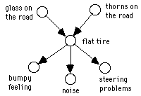
Figure 1: Example of causal graph.
A general principle for good pedagogic strategy is this: other things equal, make the essential principles of the subject explicit rather than tacit. We think that this principle is routinely violated in conventional instruction in statistics. Even though most of the early history of probability theory has been driven by causal considerations, the terms "cause" and "causation" have practically disappeared from statistics textbooks. Statistics curricula guide students away from the concept of causality, into remembering perhaps the cliche disclaimer "correlation does not mean causation," but rarely thinking about what correlation does mean. The treatment of causality is a serious handicap to later studies of such topics as experimental design, where often the main goal is to establish (or disprove) causation. Much of the technical vocabulary of the language used in research design textbooks consists in euphemisms for specific causal relations, e.g, "latent variable," "intervening variable," "confounding factor," etc. The multiplicity of terms used to refer to causation results in confusion and, in effect, may hinder understanding of the basic principles of research design.
Defining causality is at least as hard as defining probability; neither idea requires a philosophically strict definition in order for students to learn how to use the notions well. As with an understanding of probability, an understanding of causality is best promoted by examples and formal principles in combination.
In this paper, we describe our efforts to reintroduce causation in teaching research design. We show how causal graphs can be used to explain various elements of empirical research, and we report our classroom experiences with this approach.
Causal graphs are directed acyclic graphs, in which vertices denote variable features of a system and edges denote direct causal relations between these features. The joint probability distribution over the variables in a causal graph satisfies causal Markov condition [3], which says, in effect, that a variable X is independent of any variable it does not affect, conditional on values of the immediate causes of X. For example, given that the drive shaft of an engine does not turn, the motion of an axle of the same car is independent of whether or not the spark plugs fire. Two variables A and B in a graph are probabilistically dependent if there is a directed path from one to the other of if there is a directed path to A and a directed path to B from some third variable. For example, steering problems are dependent on glass on the road because glass on the road may cause flat tire and this, in turn, may cause steering problems (Figure 1). Steering problems are also probabilistically dependent on bumpy feeling and noise, as all three are connected by a common cause, flat tire. Hearing noise makes flat tire more likely and this, in turn, increases the likelihood of steering problems. A path, and the resulting dependence, can be made inactive by conditioning on (controlling for) one of the variables on it.

|
Another useful consequence of the causal Markov condition is conditional dependence of causes given their effect. For example, glass on the road and thorns on the road, two ordinarily independent causes of a flat tire become dependent if a flat tire has actually been observed, explaining each other away [1] as possible causes of the flat tire.
The causal Markov condition also allows one to derive the consequences of external manipulation of variables in a causal graph. The manipulation theorem due to Spirtes et al. [3] states that given an external intervention on a variable A in a causal graph, we can derive the posterior probability distribution over the entire graph by simply modifying the conditional probability distribution of A. If this intervention is strong enough to set A to a specific value, we can view the intervention as the only cause of A and reflect this by removing all edges that are coming into A. Nothing else in the graph needs to be modified, as the causal structure of the system remains unchanged.
The Markov property is tacitly assumed throughout the design of experiments and in much of non-experimental. We have found that students understand more clearly what is at stake in research design if graphical representations are introduced from the beginning. In the remaining sections we briefly give some examples.
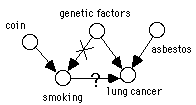
Most research design textbooks explain randomization as protection from unsuspected sources of bias. With the insight from causal graphs and especially the manipulation theorem, we can easily see that randomization serves the purpose of breaking all alternative paths from the independent variable to the dependent variable. Imagine a randomized controlled study of the effect of tobacco smoking on the incidence of lung cancer (Figure 2). A flip of a coin determines whether a subject will be in the treatment group (smokers) or the control group (non-smokers). The coin is now the only cause of smoking. All other causes of smoking, such as possible genetic predisposition shown in the graph, are made inactive -- the edges in the graph coming into smoking are, according to the manipulation theorem, broken. If the incidence of lung cancer among the smokers is higher than in non-smokers (i.e., lung cancer is probabilistically dependent on smoking), it can be attributed to a causal influence of smoking on lung cancer. It is also clear from the graph that additional variables that impact either the independent variable or the dependent variable alone (such as exposure to asbestos in Figure 2) although contribute to variability in measurements, do not disturb in drawing causal conclusions from the experiment.
|
Graphical models show what happens when there is no randomization, or when the randomization is not perfect. If there exists a variable that causes both the independent and the dependent variable (perhaps in combination with a coin), there is an alternative path between the independent and the dependent variables. An example of such situation is assigning elementary school students to various reading groups based on a pretest of their intelligence or on how assertive their parents are in having them assigned to the "best" group.
As the existence of a common cause between the independent and the dependent variables provides an alternative path between them, it provides an alternative hypothesis accounting for possible probabilistic dependence between them. The experiment is weaker in demonstrating causality. For example, in the smoking experiment, if no randomization takes place, possible genetic predisposition influencing both predisposition to smoke and to get lung cancer, is an alternative explanation for dependence between smoking and lung cancer.
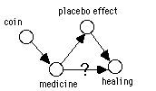
The concept of placebo in experimental design has a similarly intuitive explanation. Obtaining a medicine causes healing in itself and that impacts the dependent variable, resulting in possible dependence between independent and dependent variables even without a direct link between them (Figure 3 left). Administration of placebo to the control group makes the causal structure for the placebo path the same for both both groups and the placebo effect can be easily isolated from the effect of medicine.
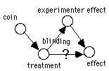
In case of subject-experimenter effects (Figure 3 right), the experimenter knows whether the subject is in the treatment group or the control group. This knowledge modifies the experimenter's behavior so that it impacts the dependent variable. Blinding removes the link from treatment to experimenter effect and assures that possible dependence is the result of a direct link between the independent and dependent variables.
|
|
We believe that an explicit representation of causal interactions in the design of empirical studies is valuable for several reasons. The foremost is that a clear model of an experiment aids in comprehending it, understanding possible weaknesses in the design, and communicating about it with other researchers. A causal model explicates the idea that joint probability distribution from which the experimental measurements will be sampled is shaped by the mechanisms working in the system, and by the uncertainty introduced by exogenous and latent variables. Since it is such mechanisms that experimental designs are trying to discover, this is consistent with the overall goal of experimentation. This approach allows the student to understand the scope of experimental design, exemplifies the importance of assumptions, and shows that there is a variety of methods and inferences by which the structure of the system can be discovered (e.g., causal discovery from observation [3]).
One of us (Druzdzel) introduced the concept of causal graphs in an introductory graduate research design course in the Department of Information Science at the University of Pittsburgh. The students had little previous experience with statistical analysis. We have not measured the impact that it had on our students and can offer only anecdotal evidence at this time. The students seem to find the causal graphs valuable. Class discussions of even most difficult topics are lively. Several of the students have spontaneously drawn causal graphs when explaining their homework exercises, although they were not prompted for doing so. The homeworks are peer reviewed, and several of the reviewers have spontaneously drawn causal graphs where they were not provided by the author. Two of the twelve students in class reported using causal graphs when talking with people outside the class on matters unrelated to the class material.
One of the reasons why causal graphs might be so useful is that they replace long verbose descriptions of experimental designs with simple and clear pictures. There is overwhelming evidence that causality is deeply rooted in human reasoning and this is not different for researchers. A clear graph in front of the eyes extends significantly the capacity of the working memory and allows to reason about matters of increased complexity [2]. Various ways in which an experiment may be flawed can be read directly from the graph. We believe that causal graphs can prove also very useful in an introductory class in statistics.
We discovered that it pays off to spend extra time in the beginning of the course to make sure that the students understand causal graphs and the causal Markov condition well. After some training, students are proficient with reasoning about probabilistic dependence and independence in graphs.
[1] Marek J. Druzdzel and Max Henrion. Intercausal reasoning with uninstantiated ancestor nodes. In Proceedings of the Ninth Annual Conference on Uncertainty in Artificial Intelligence (UAI-93), pages 317-325, Washington, D.C., 1993.